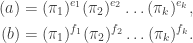
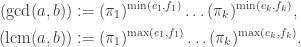
Unique Factorization
Through this article and the next few ones, we will explore unique factorization in rings. The inspiration, of course, comes from ℤ. Here is an application of unique factorization. Warning: not all steps may make sense to the reader at this point of time.
Sample Problem.
Find all integer solutions to  .
.
Solution (Sketch)
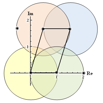
Factor the equation to obtain  where
where  . Use the fact that
 ![\mathbb Z[\alpha]](https://s0.wp.com/latex.php?latex=%5Cmathbb+Z%5B%5Calpha%5D&bg=ffffff&fg=333333&s=0&c=20201002) satisfies unique factorization; deduce that
satisfies unique factorization; deduce that  and
and  must be coprime (since x, y are odd). Hence
  and
and  for some
 ![a,b \in \mathbb Z[\alpha]](https://s0.wp.com/latex.php?latex=a%2Cb+%5Cin+%5Cmathbb+Z%5B%5Calpha%5D&bg=ffffff&fg=333333&s=0&c=20201002) with
with  . This gives
  . Now we factor
  in all possible ways and solve a pair of simultaneous equations in a and b. E.g.

which gives  ♦
♦
Before starting, here are some preliminary definitions.
Throughout this article, A denotes an integral domain.
Definition.
Recall that A is a unit if it is invertible under product.
- Elements
 are associated (written as
  ) if there is a unit
  such that
  .
.
- For we say x divides y (written as
 ) if there exists
  such that
  .
.
- Let
 ,
,  not a unit. We say it is reducible if we can find
  which are non-unit such that
  . Otherwise, is irreducible.
All the above conditions can be expressed in terms of ideals.
- x and y are associated if and only if (x) = (y) as ideals of A. Thus, the relation is an equivalence relation.
- x divides y if and only if
 as ideals. Thus and
  if and only if .
- x is irreducible if and only if when (x) = (y)(z) as a product of ideals, either (x) = (y) or (x) = (z). In particular, if x is irreducible, so are all its associates.
The descriptions in terms of principal ideals are much cleaner.
Examples
1. Suppose ![A = \mathbb Z[i] = \{a + b\sqrt{-1} : a,b\in \mathbb Z\}](https://s0.wp.com/latex.php?latex=A+%3D+%5Cmathbb+Z%5Bi%5D+%3D+%5C%7Ba+%2B+b%5Csqrt%7B-1%7D+%3A+a%2Cb%5Cin+%5Cmathbb+Z%5C%7D&bg=ffffff&fg=333333&s=0&c=20201002) . The only units are {-1, +1, –i, +i}. So each non-zero element has 4 associates, e.g.
. The only units are {-1, +1, –i, +i}. So each non-zero element has 4 associates, e.g.
 are associates,
  are associates.
Note that 1 + 2i and 1 – 2i are not associates. On the other hand, 1 + i and 1 – i are associates. (Verify this!)
2. Suppose ![A = \mathbb Z[\sqrt 2] = \{a + b\sqrt 2 : a,b \in \in \mathbb Z\}](https://s0.wp.com/latex.php?latex=A+%3D+%5Cmathbb+Z%5B%5Csqrt+2%5D+%3D+%5C%7Ba+%2B+b%5Csqrt+2+%3A+a%2Cb+%5Cin+%5Cin+%5Cmathbb+Z%5C%7D&bg=ffffff&fg=333333&s=0&c=20201002) . The unit group is infinite since it contains
. The unit group is infinite since it contains  for all
  . Thus every non-zero element has infinitely many associates.

Factoring Into Irreducibles
Let  be non-zero, non-unit. If x is reducible, we can factor it as x = yz where y, z are non-zero and non-unit. Again, if either of them is reducible, we factor them further. If this process terminates, we obtain x as a factor of irreducibles.
Unfortunately, there are cases where it does not.
Example
Let ![A = \mathbb R[x^{1/n} : n = 1, 2, \ldots]](https://s0.wp.com/latex.php?latex=A+%3D+%5Cmathbb+R%5Bx%5E%7B1%2Fn%7D+%3A+n+%3D+1%2C+2%2C+%5Cldots%5D&bg=ffffff&fg=333333&s=0&c=20201002) . Now can be factorized indefinitely:
. Now can be factorized indefinitely:

Here is a condition which ensures that factorization terminates.
Proposition 1.
Partially order the principal ideals of A by reverse inclusion:
 .
.
If this poset is noetherian, then every non-unit  can be factored as a product of irreducibles.
Note
By proposition 1 here, the above condition is equivalent to either of the following.
- Any non-empty collection of principal ideals of A has a maximal element.
- In any chain of principal ideals
 of A, there exists n such that
  .
.
One also says A satisfies ascending chain condition (a.c.c.) on the set of principal ideals.
Proof
Let S be the collection of all non-unit which cannot be factored as a product of irreducibles. If S is non-empty, the set of principal ideals (x) for  has a maximal element (z) with respect to ⊆.
Since z cannot be factored as a product of irreducibles, it is not irreducible. Write z = xy where x, y are non-unit and non-zero. Then  and
and  so by maximality of (z) we have
  . Hence x and y can be expressed as a product of finitely many irreducibles; since z = xy so does z, a contradiction. ♦
But how does one check the above abstract condition for a ring A? There are two answers to this.
- Most rings we are interested in actually satisfy a.c.c. on all ideals. Called noetherian rings, we will see later that they are everywhere.
- More immediately, we will give a criterion for unique factorizability which also implies a.c.c. on principal ideals.
UFDs
Finally, here is our main object of interest.
Definition.
An integral domain A is called a unique factorization domain (UFD) if every proper principal ideal  can be factored as a product of irreducible principal ideals.

uniquely up to permutation.
Here is a non-example. Suppose ![A = \mathbb Z[\sqrt{-5}]](https://s0.wp.com/latex.php?latex=A+%3D+%5Cmathbb+Z%5B%5Csqrt%7B-5%7D%5D&bg=ffffff&fg=333333&s=0&c=20201002) . In this ring, we have
. In this ring, we have

It is easy to see that no two of these elements are associates. Thus to see that unique factorization fails, it remains to show all of them are irreducible. For that, take the norm function  where
where  An easy calculation shows:
Now the above elements have norms

If any of them had a proper factor, such a factor would have norm 2 or 3. But it is easy to see no element of norm 2 or 3 exists.
Exercise A
Prove that ![\mathbb Z[\sqrt{10}]](https://s0.wp.com/latex.php?latex=%5Cmathbb+Z%5B%5Csqrt%7B10%7D%5D&bg=ffffff&fg=333333&s=0&c=20201002) is not a UFD.
is not a UFD.
Prime Elements
We end this section by stating a necessary and sufficient condition for unique factorization to hold.
Definition.
Let . We say x is prime if  is a prime ideal of A.
Thus x is prime if and only if:
- whenever yz is a multiple of x, either y or z is a multiple of x.
Lemma 1.
A prime element is irreducible.
Proof
Suppose x = yz, where y, z are non-zero. Then yz is a multiple of x so either y or z is a multiple of x. Assume the former, so y is a multiple of x, but since x = yz we have x is a multiple of y also. Thus x and y are associates and z is a unit. ♦
Finally, the main result we want is as follows.
Theorem 1.
Let A be a domain which satisfies a.c.c. on principal ideals.
Then A is a unique factorization domain if and only if all irreducible elements are prime.
Proof
(⇒) Let A be a UFD and be irreducible. To show x is prime, suppose  and
and  ; we need to show
  . Write
  for some
  . Write y, z and a as a product of irreducibles. By unique factorization, since x does not occur in the factoring of y, it must occur in the factoring of z. Thus .
(⇐) Suppose all irreducibles are prime. For any , suppose we have factorizations  where
where  are all irreducible, and hence prime. Write this in terms of principal ideals:

Now since  , one of the terms, say
  must be in
  . Hence is a multiple of
  ; by irreducibility we have
  . So and are associates and upon division we have

Repeat until we run out of terms on one side so we get (1). The other side must also be empty so we have established unique factorization. ♦
In the next article, we will find many examples of UFDs based on this criterion.
Example
Let us show that ![A = \mathbb Z[\sqrt {-5}]](https://s0.wp.com/latex.php?latex=A+%3D+%5Cmathbb+Z%5B%5Csqrt+%7B-5%7D%5D&bg=ffffff&fg=333333&s=0&c=20201002) is not a UFD by finding an irreducible element which is not prime: 2. By the norm argument above, 2 is irreducible but it is not prime because
is not a UFD by finding an irreducible element which is not prime: 2. By the norm argument above, 2 is irreducible but it is not prime because
![A/(2) = \mathbb Z[X]/(X^2 + 5, 2) = \mathbb F_2[X]/(X^2 + 5) = \mathbb F_2[X]/(X^2 + 1)](https://s0.wp.com/latex.php?latex=A%2F%282%29+%3D+%5Cmathbb+Z%5BX%5D%2F%28X%5E2+%2B+5%2C+2%29+%3D+%5Cmathbb+F_2%5BX%5D%2F%28X%5E2+%2B+5%29+%3D+%5Cmathbb+F_2%5BX%5D%2F%28X%5E2+%2B+1%29&bg=ffffff&fg=333333&s=0&c=20201002)
is not an integral domain.
Exercise B
Find all prime ideals of which contain 2 or 3.
[Hint (highlight to read): prime ideals of A containing 2 correspond to prime ideals of A/(2).]

, where
.


![\mathbb Q[\sqrt{-1}]](https://s0.wp.com/latex.php?latex=%5Cmathbb+Q%5B%5Csqrt%7B-1%7D%5D&bg=ffffff&fg=333333&s=0&c=20201002)
![\mathbb Z[\sqrt{-1}]](https://s0.wp.com/latex.php?latex=%5Cmathbb+Z%5B%5Csqrt%7B-1%7D%5D&bg=ffffff&fg=333333&s=0&c=20201002)
![k[X]](https://s0.wp.com/latex.php?latex=k%5BX%5D&bg=ffffff&fg=333333&s=0&c=20201002)

![f(X), g(X)\in k[X]](https://s0.wp.com/latex.php?latex=f%28X%29%2C+g%28X%29%5Cin+k%5BX%5D&bg=ffffff&fg=333333&s=0&c=20201002)


can be uniquely written as
,
and
. We call this the prime factorization of


, equivalently
for each
.
.
.


is a UFD, so is its ring of polynomials
.
![f \in A[X] - \{0\}](https://s0.wp.com/latex.php?latex=f+%5Cin+A%5BX%5D+-+%5C%7B0%5C%7D&bg=ffffff&fg=333333&s=0&c=20201002)

![A[X]/(\pi) \cong (A/\pi)[X]](https://s0.wp.com/latex.php?latex=A%5BX%5D%2F%28%5Cpi%29+%5Ccong+%28A%2F%5Cpi%29%5BX%5D&bg=ffffff&fg=333333&s=0&c=20201002)
![f = a_0 + a_1 X + \ldots \in A[X]](https://s0.wp.com/latex.php?latex=f+%3D+a_0+%2B+a_1+X+%2B+%5Cldots+%5Cin+A%5BX%5D&bg=ffffff&fg=333333&s=0&c=20201002)
![g = b_0 + b_1 X + \ldots \in A[X]](https://s0.wp.com/latex.php?latex=g+%3D+b_0+%2B+b_1+X+%2B+%5Cldots+%5Cin+A%5BX%5D&bg=ffffff&fg=333333&s=0&c=20201002)
.
; similarly, there is a maximum e such that
.
in fg is not a multiple of

![g \in K[X] - \{0\}](https://s0.wp.com/latex.php?latex=g+%5Cin+K%5BX%5D+-+%5C%7B0%5C%7D&bg=ffffff&fg=333333&s=0&c=20201002)


![p(g) \in A[X]](https://s0.wp.com/latex.php?latex=p%28g%29+%5Cin+A%5BX%5D&bg=ffffff&fg=333333&s=0&c=20201002)


![g = c(g)p(g), \quad c(g)\in K^*, p(g) \in A[X] \text{ primitive.}](https://s0.wp.com/latex.php?latex=g+%3D+c%28g%29p%28g%29%2C+%5Cquad+c%28g%29%5Cin+K%5E%2A%2C+p%28g%29+%5Cin+A%5BX%5D+%5Ctext%7B+primitive.%7D&bg=ffffff&fg=333333&s=0&c=20201002)


![p\in A[X]](https://s0.wp.com/latex.php?latex=p%5Cin+A%5BX%5D&bg=ffffff&fg=333333&s=0&c=20201002)


![f = c(f)p(f), \ g = c(g)p(g), \quad c(f), c(g)\in K^*, p(f), p(g) \in A[X] \text{ primitive.}](https://s0.wp.com/latex.php?latex=f+%3D+c%28f%29p%28f%29%2C+%5C+g+%3D+c%28g%29p%28g%29%2C+%5Cquad+c%28f%29%2C+c%28g%29%5Cin+K%5E%2A%2C+p%28f%29%2C+p%28g%29+%5Cin+A%5BX%5D+%5Ctext%7B+primitive.%7D&bg=ffffff&fg=333333&s=0&c=20201002)


![f \in A[X]](https://s0.wp.com/latex.php?latex=f+%5Cin+A%5BX%5D&bg=ffffff&fg=333333&s=0&c=20201002)

![K[X]](https://s0.wp.com/latex.php?latex=K%5BX%5D&bg=ffffff&fg=333333&s=0&c=20201002)

![g, h\in K[X]](https://s0.wp.com/latex.php?latex=g%2C+h%5Cin+K%5BX%5D&bg=ffffff&fg=333333&s=0&c=20201002)
![f\in A[X]](https://s0.wp.com/latex.php?latex=f%5Cin+A%5BX%5D&bg=ffffff&fg=333333&s=0&c=20201002)

![g, h, h' \in A[X]](https://s0.wp.com/latex.php?latex=g%2C+h%2C+h%27+%5Cin+A%5BX%5D&bg=ffffff&fg=333333&s=0&c=20201002)


![g' \in K[X]](https://s0.wp.com/latex.php?latex=g%27+%5Cin+K%5BX%5D&bg=ffffff&fg=333333&s=0&c=20201002)

![f\in A[X] - \{0\}](https://s0.wp.com/latex.php?latex=f%5Cin+A%5BX%5D+-+%5C%7B0%5C%7D&bg=ffffff&fg=333333&s=0&c=20201002)
,
![k[X_1, \ldots, X_n]](https://s0.wp.com/latex.php?latex=k%5BX_1%2C+%5Cldots%2C+X_n%5D&bg=ffffff&fg=333333&s=0&c=20201002)
![\mathbb Z[X_1, \ldots, X_n]](https://s0.wp.com/latex.php?latex=%5Cmathbb+Z%5BX_1%2C+%5Cldots%2C+X_n%5D&bg=ffffff&fg=333333&s=0&c=20201002)


![\mathbb C[X, Y, Z]/(Z^2 - X^2 - Y^2)](https://s0.wp.com/latex.php?latex=%5Cmathbb+C%5BX%2C+Y%2C+Z%5D%2F%28Z%5E2+-+X%5E2+-+Y%5E2%29&bg=ffffff&fg=333333&s=0&c=20201002)
 are prime elements and
  are integers.
 if and only if
  .
. for
for  . If, say,
 recursively via
 ; if
; if  satisfies
  then
then  .
. ; if
; if  then
then  We often say elements
  . E.g. in the next article we will show that
 ![k[X, Y]](https://s0.wp.com/latex.php?latex=k%5BX%2C+Y%5D&bg=ffffff&fg=333333&s=0&c=20201002) is a UFD but (X, Y) is a proper ideal.
is a UFD but (X, Y) is a proper ideal. be a chain of principal ideals of A. Now the union of an ascending chain of ideals is an ideal (see
  is an ideal, necessarily principal. Write
  . Then
  for some n. So
 . This proves the first claim
 is principal so we write
  . Thus x is a multiple of y’; since x is irreducible this means either (x) = (y’) or y’ is a unit.
 .
. for some
  so
so  since
since  such that
 where
where  , we can write
  for some
  such that
  or
or  .
. be an ideal. If
  it is clearly principal. Otherwise, pick
  such that
  is minimum. We claim that
  Clearly we only need to show ⊆.
 . Thus we can write
  where
where  . In the former case we have
  . The latter case cannot happen since
  ,
,  . Thus
  . ♦
. ♦
![A = k[X]](https://s0.wp.com/latex.php?latex=A+%3D+k%5BX%5D&bg=ffffff&fg=333333&s=0&c=20201002) , where k is a field. We take the degree of a polynomial
, where k is a field. We take the degree of a polynomial
 , the remainder theorem gives
  where
where  or
or  . This is exactly the condition for an Euclidean function.
![A = \mathbb Z[\sqrt{-1}]](https://s0.wp.com/latex.php?latex=A+%3D+%5Cmathbb+Z%5B%5Csqrt%7B-1%7D%5D&bg=ffffff&fg=333333&s=0&c=20201002) given by
given by 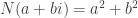 is Euclidean. Note that N extends to
![N : \mathbb Q[\sqrt{-1}] = \{a + bi : a,b\in \mathbb Q\} \longrightarrow \mathbb Q, \quad N(a+bi) = a^2 + b^2](https://s0.wp.com/latex.php?latex=N+%3A+%5Cmathbb+Q%5B%5Csqrt%7B-1%7D%5D+%3D+%5C%7Ba+%2B+bi+%3A+a%2Cb%5Cin+%5Cmathbb+Q%5C%7D+%5Clongrightarrow+%5Cmathbb+Q%2C+%5Cquad+N%28a%2Bbi%29+%3D+a%5E2+%2B+b%5E2&bg=ffffff&fg=333333&s=0&c=20201002)
![a,b\in \mathbb Z[\sqrt{-1}]](https://s0.wp.com/latex.php?latex=a%2Cb%5Cin+%5Cmathbb+Z%5B%5Csqrt%7B-1%7D%5D&bg=ffffff&fg=333333&s=0&c=20201002) with
with ![x = \frac a b \in \mathbb Q[\sqrt{-1}]](https://s0.wp.com/latex.php?latex=x+%3D+%5Cfrac+a+b+%5Cin+%5Cmathbb+Q%5B%5Csqrt%7B-1%7D%5D&bg=ffffff&fg=333333&s=0&c=20201002) . By rounding off the real and imaginary parts of x, we obtain
. By rounding off the real and imaginary parts of x, we obtain ![q\in \mathbb Z[\sqrt{-1}]](https://s0.wp.com/latex.php?latex=q%5Cin+%5Cmathbb+Z%5B%5Csqrt%7B-1%7D%5D&bg=ffffff&fg=333333&s=0&c=20201002) such that
such that
 . Hence we have:
 .
. be prime..
 we have
  , where
  is prime.
 , then p is still prime in A.
 , then
  where
where  are primes which are not associates.
![A/(p) \cong \mathbb Z[X]/(X^2 + 1, p) \cong \mathbb F_p[X]/(X^2 + 1).](https://s0.wp.com/latex.php?latex=A%2F%28p%29+%5Ccong+%5Cmathbb+Z%5BX%5D%2F%28X%5E2+%2B+1%2C+p%29+%5Ccong+%5Cmathbb+F_p%5BX%5D%2F%28X%5E2+%2B+1%29.&bg=ffffff&fg=333333&s=0&c=20201002)
 has no solution. From theory of quadratic residues, this holds if and only if
  . For
. For  , we have
![A/(p) \cong F_p[X]/((X - u)(X-v))](https://s0.wp.com/latex.php?latex=A%2F%28p%29+%5Ccong+F_p%5BX%5D%2F%28%28X+-+u%29%28X-v%29%29&bg=ffffff&fg=333333&s=0&c=20201002)
 ; hence in the original ring A we have
  since X corresponds to i. And since A is a PID, we have
  .
. in each of the following cases:
 is the norm of
 ![x+ yi \in \mathbb Z[\sqrt{-1}]](https://s0.wp.com/latex.php?latex=x%2B+yi+%5Cin+%5Cmathbb+Z%5B%5Csqrt%7B-1%7D%5D&bg=ffffff&fg=333333&s=0&c=20201002) .]
.]![\mathbb Z[\sqrt{-2}], \ \ \mathbb Z[\frac{1 + \sqrt{-3}} 2], \ \ \mathbb Z[\frac{1 + \sqrt{-7}}2], \ \ \mathbb Z[\frac{1 + \sqrt{-11}}2].](https://s0.wp.com/latex.php?latex=%5Cmathbb+Z%5B%5Csqrt%7B-2%7D%5D%2C+%5C+%5C+%5Cmathbb+Z%5B%5Cfrac%7B1+%2B+%5Csqrt%7B-3%7D%7D+2%5D%2C+%5C+%5C+%5Cmathbb+Z%5B%5Cfrac%7B1+%2B+%5Csqrt%7B-7%7D%7D2%5D%2C+%5C+%5C+%5Cmathbb+Z%5B%5Cfrac%7B1+%2B+%5Csqrt%7B-11%7D%7D2%5D.&bg=ffffff&fg=333333&s=0&c=20201002)
 for positive integers x and n.
 ,
, for all x,
 .
. , let
, let  , an open subset of Spec A. Note that
 .
. over all
  .
. be an open subset of Spec A. Suppose
  so that
  . Pick an
  . Since
  we have
  . It remains to show
  . Indeed if
  then certainly
  so we have
  . ♦
. ♦ is a basic open covering; we need to show there is a finite subcover. Now
  where
where  , i.e. the ideal generated by the
  . This can only happen if
 so we have
 ♦
♦ for a ring A. Immediately, we see some differences between X and affine varieties. Firstly, points of X are prime ideals
  and often
  is not closed in X. More generally, we have the following.
 , the closure of
  . In particular,
  containing
  . On the other hand, any closed subset
  so
so  . Thus
  . ♦
. ♦ is the closure of the point (0). In a topological space X, a generic point of X is a
  such that the closure of
  is X.
is X. has the cofinite topology.]
 . From the
 .
. .
. for maximal ideal
  then since
  we have
  so there exists
  such that
  so
so  is not a unit, i.e.
  .
. ; let
; let  , or else we would have
  . ♦
. ♦ .
. be a product of rings. Then
  and
and  .
. where V, W are disjoint closed subsets, then
 .
. gives continuous map
  which takes
  . This map is injective, continuous and takes closed set
  to closed set
  . Hence it is a subspace embedding.
 ; by
; by  and
and  so
so
 ; pick
  ,
,  such that
  so (x) and (y) are
  which is contained in the nilradical since it is contained in all prime ideals. Thus
  for some n > 0 so
  are coprime ideals with product zero. By
  .
. we have
  ; similarly
  . Since
  and
and  also form a disjoint union of Spec A by the first part, we are done. ♦
 . Then
 . ♦
. ♦ is irreducible then it has a generic point.
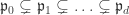
![A = k[X, Y]](https://s0.wp.com/latex.php?latex=A+%3D+k%5BX%2C+Y%5D&bg=ffffff&fg=333333&s=0&c=20201002) for a field X, we have
for a field X, we have  which is a prime chain of length 2.
![\dim A[X] \ge \dim A + 1](https://s0.wp.com/latex.php?latex=%5Cdim+A%5BX%5D+%5Cge+%5Cdim+A+%2B+1&bg=ffffff&fg=333333&s=0&c=20201002) , since for any prime chain
, since for any prime chain  of A, we have the prime chain of A[X]:
![\mathfrak p_0[X] \subsetneq \mathfrak p_1[X] \subsetneq \ldots \subsetneq \mathfrak p_d[X] \subsetneq \mathfrak p_d[X] + (X).](https://s0.wp.com/latex.php?latex=%5Cmathfrak+p_0%5BX%5D+%5Csubsetneq+%5Cmathfrak+p_1%5BX%5D%C2%A0+%5Csubsetneq+%5Cldots+%5Csubsetneq+%5Cmathfrak+p_d%5BX%5D+%5Csubsetneq+%5Cmathfrak+p_d%5BX%5D+%2B+%28X%29.&bg=ffffff&fg=333333&s=0&c=20201002)
![A[X]/\mathfrak p_i[X] \cong (A/\mathfrak p_i)[X]](https://s0.wp.com/latex.php?latex=A%5BX%5D%2F%5Cmathfrak+p_i%5BX%5D+%5Ccong+%28A%2F%5Cmathfrak+p_i%29%5BX%5D&bg=ffffff&fg=333333&s=0&c=20201002) and
and ![A[X]/(\mathfrak p_d[X] +(X)) \cong A/\mathfrak p_d](https://s0.wp.com/latex.php?latex=A%5BX%5D%2F%28%5Cmathfrak+p_d%5BX%5D+%2B%28X%29%29+%5Ccong+A%2F%5Cmathfrak+p_d&bg=ffffff&fg=333333&s=0&c=20201002) .
.![\dim k[X_1, \ldots, X_n] \ge n](https://s0.wp.com/latex.php?latex=%5Cdim+k%5BX_1%2C+%5Cldots%2C+X_n%5D+%5Cge+n&bg=ffffff&fg=333333&s=0&c=20201002) and
and ![\dim \mathbb Z[X_1, \ldots, X_n] \ge n+1](https://s0.wp.com/latex.php?latex=%5Cdim+%5Cmathbb+Z%5BX_1%2C+%5Cldots%2C+X_n%5D+%5Cge+n%2B1&bg=ffffff&fg=333333&s=0&c=20201002) . Eventually, we will see that equality holds!
. Eventually, we will see that equality holds! .
.![\mathfrak m\subset k[V]](https://s0.wp.com/latex.php?latex=%5Cmathfrak+m%5Csubset+k%5BV%5D&bg=ffffff&fg=333333&s=0&c=20201002) . For general rings, we have to switch to taking prime ideals because of the following.
. For general rings, we have to switch to taking prime ideals because of the following. is a ring homomorphism and
  is a prime ideal of B, then
  is a prime ideal of A.
 has kernel
  . Hence this induces an injective ring homomorphism
  . Since
  is a domain, so is
  so
so  . The zero ideal is maximal in
  is not maximal in
  is closed if and only if it is of the following form
 .
. where
where  of A and ideals
  of A, we have
 ,
, ,
, .
. for each i if and only if it contains
  .
. and
and  so we have
 . Then
  and
and  so there are
  and
and  . Then
  since
since  . Hence if
  then
then  . ♦
. ♦ is contained in a maximal ideal.
 be the collection of all proper ideals
  containing
  has an upper bound. Since
  we may assume without loss of generality
  .
. . Let us show that
  is an ideal of A.
 . Let
. Let  and
and  and
and  for some
  . Since
  is totally ordered, either
  or
or  . Assuming the former, this gives
  so
so  . Thus
  contains 1, we have
  . Hence
  is an upper bound of
  contains a minimal prime
  if
if  . To apply Zorn’s lemma we need to show that every chain
  has a maximal element (i.e. minimal with respect to inclusion). Without loss of generality we may assume
  .
. , an ideal of A. We need to show that it is prime. Suppose
  so there exist
  such that
  and
and  . Since
  or
or  ; assuming the former we have
  . Since
  is prime we have
  so
so  .
. is a ring homomorphism. We saw that this induces a map
 .
. is continuous with respect to the Zariski topology; in fact
 is not an ideal of B in general, but that is okay since we defined V on arbitrary subsets.
 . This lies in the LHS if and only if
  contains
  we have
 induces
 ,
, contains
  . Since
  .
. not containing any power of x; thus
  .
. with
with  . Now
. Now  and
and  strictly contain
  . Hence
 and
and  in Spec A, write down the corresponding operations for radical ideals of A.
 .
. , if
, if  and
and  , then
  .
. , if
, if  , then
  .
. , either
  , for
, for  , we write:
 if
if  ;
; if
if  ;
; if
if  .
. .
. such that for any
  .
. such that for any
  .
. such that for any
  then
then  .
. such that for any
  then
then  .
.
 . Must
  , we have
  ).
). under the arithmetic ordering, the subset T of even integers has no upper or lower bound. The subset T’ of squares has lower bounds 0, -1, -2, … but no upper bound.
 be any non-empty subset. Pick
  . If
. If  is a minimal element of T we are done; otherwise there exists
  ,
,  . Again if
  in T. Thus T has a minimal element.
 of positive integers under ≤ is noetherian.
 is noetherian, where
  if
if  and
and  .
. to mean
  .
. , then
  .
. ,
,  is non-empty so it has a minimal element x. By minimality, any
  with
with  in S, there is an n such that
  .
. thus has a minimal element
  . Since we have
  , equality must hold by minimality.
 with
with  . Again since
  is not minimal we can find
  with
with  . Repeat to obtain an infinitely decreasing sequence. ♦
 . Using Zorn’s lemma, one can show that a basis exists but describing it does not seem possible. Generally, results that require Zorn’s lemma are of this nature: they claim existence of certain objects or constructions without exhibiting them explicitly. Some of these are rather unnerving, like the
  ,
,  if and only if
  . Next, we claim that every chain
  ; we need to show that D is a linearly independent subset of V, so that
  is an upper bound of
 , we have
  for some
  . But
. But  for all
  ; since
  is linearly independent, we have
  .
. outside the span of C. This means
  is linearly independent, thus contradicting the maximality of C. ♦
 is identified by its coordinate ring k[V], which is a finitely generated k-algebra since
![k[V] = k[X_1, \ldots, X_n] / I(V).](https://s0.wp.com/latex.php?latex=k%5BV%5D+%3D+k%5BX_1%2C+%5Cldots%2C+X_n%5D+%2F+I%28V%29.&bg=ffffff&fg=333333&s=0&c=20201002)
![A = k[V]](https://s0.wp.com/latex.php?latex=A+%3D+k%5BV%5D&bg=ffffff&fg=333333&s=0&c=20201002) for the algebra instead.
for the algebra instead. is a homomorphism of the corresponding k-algebras
 ![f^* : k[W] \to k[V].](https://s0.wp.com/latex.php?latex=f%5E%2A+%3A+k%5BW%5D+%5Cto+k%5BV%5D.&bg=ffffff&fg=333333&s=0&c=20201002)
 .
.![k[X_1, \ldots, X_n] \to A](https://s0.wp.com/latex.php?latex=k%5BX_1%2C+%5Cldots%2C+X_n%5D+%5Cto+A&bg=ffffff&fg=333333&s=0&c=20201002) ; its kernel
; its kernel ![A \cong k[V(\mathfrak a)]](https://s0.wp.com/latex.php?latex=A+%5Ccong+k%5BV%28%5Cmathfrak+a%29%5D&bg=ffffff&fg=333333&s=0&c=20201002) . ♦
. ♦
 . The advantage here is that now we can expand the class of objects of interest.
![k[V]](https://s0.wp.com/latex.php?latex=k%5BV%5D&bg=ffffff&fg=333333&s=0&c=20201002) is reduced.
is reduced. is a maximal ideal of k[V]; equivalently we have a k-algebra homomorphism
 ![k[V] \to k](https://s0.wp.com/latex.php?latex=k%5BV%5D+%5Cto+k&bg=ffffff&fg=333333&s=0&c=20201002) .
. is a morphism of affine k-schemes.
![\phi^* : k[W] \to k[V]](https://s0.wp.com/latex.php?latex=%5Cphi%5E%2A+%3A+k%5BW%5D+%5Cto+k%5BV%5D&bg=ffffff&fg=333333&s=0&c=20201002) is a homomorphism of k-algebras.
is a homomorphism of k-algebras.![k[W] = k[V] /\mathfrak a](https://s0.wp.com/latex.php?latex=k%5BW%5D+%3D+k%5BV%5D+%2F%5Cmathfrak+a&bg=ffffff&fg=333333&s=0&c=20201002) for some radical ideal
for some radical ideal ![k[W] = k[V]/\mathfrak p](https://s0.wp.com/latex.php?latex=k%5BW%5D+%3D+k%5BV%5D%2F%5Cmathfrak+p&bg=ffffff&fg=333333&s=0&c=20201002) for some prime ideal
for some prime ideal  is a set-theoretic intersection in V.
![k[W_i] = k[V] / \mathfrak a_i](https://s0.wp.com/latex.php?latex=k%5BW_i%5D+%3D+k%5BV%5D+%2F+%5Cmathfrak+a_i&bg=ffffff&fg=333333&s=0&c=20201002) , we have
, we have ![k[W] = k[V] / r(\sum_i \mathfrak a_i)](https://s0.wp.com/latex.php?latex=k%5BW%5D+%3D+k%5BV%5D+%2F+r%28%5Csum_i+%5Cmathfrak+a_i%29&bg=ffffff&fg=333333&s=0&c=20201002) .
. is a union in V.
![k[W_i] = k[V]/\mathfrak a_i](https://s0.wp.com/latex.php?latex=k%5BW_i%5D+%3D+k%5BV%5D%2F%5Cmathfrak+a_i&bg=ffffff&fg=333333&s=0&c=20201002) , we have
, we have ![k[W] = k[V]/(\mathfrak a_1 \cap \mathfrak a_2)](https://s0.wp.com/latex.php?latex=k%5BW%5D+%3D+k%5BV%5D%2F%28%5Cmathfrak+a_1+%5Ccap+%5Cmathfrak+a_2%29&bg=ffffff&fg=333333&s=0&c=20201002) .
.![k[W] = k[V]/\mathfrak a](https://s0.wp.com/latex.php?latex=k%5BW%5D+%3D+k%5BV%5D%2F%5Cmathfrak+a&bg=ffffff&fg=333333&s=0&c=20201002) for some ideal
for some ideal ![k[W] = k[V] / (\sum_i \mathfrak a_i)](https://s0.wp.com/latex.php?latex=k%5BW%5D+%3D+k%5BV%5D+%2F+%28%5Csum_i+%5Cmathfrak+a_i%29&bg=ffffff&fg=333333&s=0&c=20201002) .
. must be of the form
  , where
  ) is an ideal of A (resp. B).
 or
or  , where
  or
or  , where
  ) is a maximal ideal of A (resp. B).
 in the above table.
 is just
 ![k[*] = k](https://s0.wp.com/latex.php?latex=k%5B%2A%5D+%3D+k&bg=ffffff&fg=333333&s=0&c=20201002) . A point on an affine k-scheme V is thus a morphism
. A point on an affine k-scheme V is thus a morphism  .
.![k[\#] := k[X]/(X^2)](https://s0.wp.com/latex.php?latex=k%5B%5C%23%5D+%3A%3D+k%5BX%5D%2F%28X%5E2%29&bg=ffffff&fg=333333&s=0&c=20201002) . We will write this as
. We will write this as ![k[\#] = k[\epsilon]](https://s0.wp.com/latex.php?latex=k%5B%5C%23%5D+%3D+k%5B%5Cepsilon%5D&bg=ffffff&fg=333333&s=0&c=20201002) with
with  . Geometrically,
  corresponds to a “small perturbation” such that
  ; the corresponding homomorphism
 ![k[\epsilon] \to k](https://s0.wp.com/latex.php?latex=k%5B%5Cepsilon%5D+%5Cto+k&bg=ffffff&fg=333333&s=0&c=20201002) takes
takes  .
. takes the point to a point P on V and the arrow to a tangent vector at P.
 .
. is given by composing
  . The tangent space of a point
  is the set of all tangent vectors with base point P, denoted by
  .
.![\phi^* : k[V] \to k[\epsilon] = k[X]/(X^2)](https://s0.wp.com/latex.php?latex=%5Cphi%5E%2A+%3A+k%5BV%5D+%5Cto+k%5B%5Cepsilon%5D+%3D+k%5BX%5D%2F%28X%5E2%29&bg=ffffff&fg=333333&s=0&c=20201002) .
. has base point P, then
  in the composition
 ![k[V] \stackrel {\phi^*}\to k[\epsilon] \to k](https://s0.wp.com/latex.php?latex=k%5BV%5D+%5Cstackrel+%7B%5Cphi%5E%2A%7D%5Cto+k%5B%5Cepsilon%5D+%5Cto+k&bg=ffffff&fg=333333&s=0&c=20201002) . This means
. This means  and so
  . Thus
 ![\phi^* : k[V] \longrightarrow k[V]/\mathfrak m_P^2 \stackrel f\longrightarrow k[\epsilon].](https://s0.wp.com/latex.php?latex=%5Cphi%5E%2A+%3A+k%5BV%5D+%5Clongrightarrow+k%5BV%5D%2F%5Cmathfrak+m_P%5E2+%5Cstackrel+f%5Clongrightarrow+k%5B%5Cepsilon%5D.&bg=ffffff&fg=333333&s=0&c=20201002)
![f : k[V]/\mathfrak m_P^2 \to k[\epsilon]](https://s0.wp.com/latex.php?latex=f+%3A+k%5BV%5D%2F%5Cmathfrak+m_P%5E2+%5Cto+k%5B%5Cepsilon%5D&bg=ffffff&fg=333333&s=0&c=20201002) which satisfies
which satisfies  . This gives a k-linear map
  , i.e. the dual space of
  as a k-vector space.
 also gives a k-algebra homomorphism
 ![k[V]/\mathfrak m_P^2 \to k[\epsilon]](https://s0.wp.com/latex.php?latex=k%5BV%5D%2F%5Cmathfrak+m_P%5E2+%5Cto+k%5B%5Cepsilon%5D&bg=ffffff&fg=333333&s=0&c=20201002) by mapping k to k. Hence we have shown:
by mapping k to k. Hence we have shown: with
with ![k[V] = k[X, Y]](https://s0.wp.com/latex.php?latex=k%5BV%5D+%3D+k%5BX%2C+Y%5D&bg=ffffff&fg=333333&s=0&c=20201002) . A point
. A point  corresponds to
 ![\mathfrak m_P = (X - \alpha, Y - \beta) \subset k[X, Y]](https://s0.wp.com/latex.php?latex=%5Cmathfrak+m_P+%3D+%28X+-+%5Calpha%2C+Y+-+%5Cbeta%29+%5Csubset+k%5BX%2C+Y%5D&bg=ffffff&fg=333333&s=0&c=20201002) . A tangent vector at P then corresponds to a k-linear map
. A tangent vector at P then corresponds to a k-linear map
 is generated by
  so g is uniquely determined by
  and
and  . Clearly
  .
.![\phi^* : k[X, Y] \to k[\epsilon]](https://s0.wp.com/latex.php?latex=%5Cphi%5E%2A+%3A+k%5BX%2C+Y%5D+%5Cto+k%5B%5Cepsilon%5D&bg=ffffff&fg=333333&s=0&c=20201002) we take, for each
we take, for each ![f(X, Y) \in k[X, Y]](https://s0.wp.com/latex.php?latex=f%28X%2C+Y%29+%5Cin+k%5BX%2C+Y%5D&bg=ffffff&fg=333333&s=0&c=20201002) ,
,
 . Hence
 is cut out by
  , so
, so ![k[V] = k[X, Y]/(Y^2 - X^3 + X)](https://s0.wp.com/latex.php?latex=k%5BV%5D+%3D+k%5BX%2C+Y%5D%2F%28Y%5E2+-+X%5E3+%2B+X%29&bg=ffffff&fg=333333&s=0&c=20201002) . Take the point P = (0, 0), which corresponds to
. Take the point P = (0, 0), which corresponds to  . Let us compute the space of tangent vectors at P.
![\mathfrak m_P^2 = (X^2, XY, Y^2) \subset k[V]](https://s0.wp.com/latex.php?latex=%5Cmathfrak+m_P%5E2+%3D+%28X%5E2%2C+XY%2C+Y%5E2%29+%5Csubset+k%5BV%5D&bg=ffffff&fg=333333&s=0&c=20201002) . Instead of looking at
. Instead of looking at  as ideals of
 .
. cut out by
  so
so ![k[V] = k[X, Y]/(Y^2 - X^2 - X^3)](https://s0.wp.com/latex.php?latex=k%5BV%5D+%3D+k%5BX%2C+Y%5D%2F%28Y%5E2+-+X%5E2+-+X%5E3%29&bg=ffffff&fg=333333&s=0&c=20201002) . Take P = (0, 0) again.
. Take P = (0, 0) again.
 . Again, we take their preimages
  and
and  as ideals of
  and so
 .
. .
. .
. .
. , together with a multiplication operator
  such that
 becomes a commutative ring (with 1);
 .
. and
and  we have
 ,
,  is a ring homomorphism.
 , B takes the structure of an A-algebra, where the A-module map is:


 .
. which is also a ring homomorphism.
 . A homomorphism of A-algebras is precisely a ring homomorphism
  such that
  .
.
 . Hence for
  ,
, ♦
♦
 be the set of A-algebra homomorphisms
  . Unlike the case of modules, this set has no canonical additive structure, since if
  are homomorphisms of A-algebras,
  usually is not (e.g. it does not take 1 to 1).
![B = A[X, Y]/(XY - 1)](https://s0.wp.com/latex.php?latex=B+%3D+A%5BX%2C+Y%5D%2F%28XY+-+1%29&bg=ffffff&fg=333333&s=0&c=20201002) . Any A-algebra homomorphism
. Any A-algebra homomorphism  corresponds to a pair of elements
  such that
  . Thus we have a bijection:
 induces a map
 .
. . To express this rigorously, one needs the language of category theory.
 .
. are not just sets, but have group structures as well. To specify these group structures rigorously, one requires B to have a Hopf algebra structure.
 is a collection of subalgebras, their intersection
  is clearly also a subalgebra of B. This follows from the fact that intersection of submodules (resp. subring) is a submodule (resp. subring).
 , let
, let  is the A-subalgebra of B generated by S; it is denoted by
 ![A[S].](https://s0.wp.com/latex.php?latex=A%5BS%5D.&bg=ffffff&fg=333333&s=0&c=20201002)
 , and polynomial
 ![f(X_1, \ldots, X_k) \in A[X_1, \ldots, X_k]](https://s0.wp.com/latex.php?latex=f%28X_1%2C+%5Cldots%2C+X_k%29+%5Cin+A%5BX_1%2C+%5Cldots%2C+X_k%5D&bg=ffffff&fg=333333&s=0&c=20201002) in k variables, we take the element
in k variables, we take the element  . Taking the set of all these elements over all k, all
  and all
  then gives us
 ![A[S]](https://s0.wp.com/latex.php?latex=A%5BS%5D&bg=ffffff&fg=333333&s=0&c=20201002) .
.![B = A[S]](https://s0.wp.com/latex.php?latex=B+%3D+A%5BS%5D&bg=ffffff&fg=333333&s=0&c=20201002) for some finite subset
for some finite subset  .
. , it suffices to take only polynomials f in exactly n variables and consider all
  , in which case we have a surjective homomorphism of A-algebras
![A[X_1, \ldots, X_n] \longrightarrow B, \qquad f(X_1, \ldots, X_n) \mapsto f(\alpha_1, \ldots, \alpha_n).](https://s0.wp.com/latex.php?latex=A%5BX_1%2C+%5Cldots%2C+X_n%5D+%5Clongrightarrow+B%2C+%5Cqquad+f%28X_1%2C+%5Cldots%2C+X_n%29+%5Cmapsto+f%28%5Calpha_1%2C+%5Cldots%2C+%5Calpha_n%29.&bg=ffffff&fg=333333&s=0&c=20201002)
 be a collection of A-algebras. Let
  be the set-theoretic product; we saw
  , which is compatible with its A-module structure. Thus:
 define the projection map
 satisfies the following.
 where each
  is an A-algebra homomorphism, there is a unique A-algebra homomorphism
  such that
  for each
  .
. is the A-algebra analogue of the
  as an A-module then define multiplication component-wise, but it would not work since
  does not contain
  . The correct answer is obtained via tensor products, which will be covered in a later article.
 gives the A-module
  where the operations are defined component-wise. In this article, we will generalize the construction to an infinite collection of modules. Throughout this article, let
  denote a collection of A-modules, indexed by
  is the set-theoretic product of the
  , with the structure of an A-module given by:
 .
. is the submodule of
  such that
  only for a finite number of
  , one often writes the element additively, i.e.
  .
. for a fixed module M, then
  is the set of all functions
  . On the other hand,
  is the set of all f such that
  for only finitely many
 . For each
 satisfies the following.
 where each
  such that
  .
. “classify” the collection of all I-indexed tuples
  .
.
 to be
to be  . Now for any
  .
. is
is  so the tuple
  . ♦
. ♦ be a collection of data satisfying the above universal property. Then there is a unique isomorphism
  such that
  for all
  and
and  for each i. There exists a unique
  such that
  . We know one such f, namely
  . Hence this is the only possibility.
 . There exists a unique
  such that
  for each i.
 also satisfies this same universal property. Swapping M and M’ there exists a unique
  for each i. By step 1, we have
  . By symmetry we get
  too. ♦
 . For each
 has component
  at
at  and 0 if
  . The collection of data
  satisfies the following.
 where each
  is A-linear, there is a unique A-linear
  such that
  for each
  be a collection of data satisfying the above universal property. Then there is a unique isomorphism
  such that
  for each
  which take
  ;
; which take
  fails the universal property of direct sum, and
  fails the universal property of direct product.
 . Consider the
 are non-zero. Also,
  is independent of our choice of integer
  .
. where
where  are distinct primes and each
  . Multiplying throughout by
  gives
gives
 . Since
  is coprime to
  which is a contradiction.
 where n is square free. Indeed, suppose n in
  as a product of distinct primes.
 of G has order n.
 maps into G injectively with image with
  .
. , we see that
  .
. , let
, let  . Now, the submodule of M generated by S is:
 , the sum
  is simply the submodule of M generated by their union
  .
. consists of the set of all finite linear combinations
 for some finite subset S of M.
 where A = (1) is finitely generated but
 be the set of all sums with only positive
  . This ideal is not finitely generated, since any finite subset
  is contained in
 ![x^{1/n} \mathbb R[x^{1/n}]](https://s0.wp.com/latex.php?latex=x%5E%7B1%2Fn%7D+%5Cmathbb+R%5Bx%5E%7B1%2Fn%7D%5D&bg=ffffff&fg=333333&s=0&c=20201002) for some n > 0 so
for some n > 0 so  lies outside (S).
 is a finite subset, there is a unique A-linear
 , i.e. some of the elements may repeat.
 for some n > 0. When is f injective?
 , then all
  .
. generates M.
 are both bases, must we have
  ? This question will be answered a few articles later.
 we have
 , then treating
  as a submodule of
  we have
 as
as  to avoid cluttering up the notation.
 by
by  .
. .
. for
for  is just
  .
. via
via  , which is a well-defined homomorphism. Clearly the map is surjective; the kernel is just N/P; now apply the first isomorphism theorem. ♦
 in the first case, it corresponds to
  in the second.
 if and only if
  ;
; ;
; .
. is the largest submodule contained in every
  may not contain P. However,
  does and we have:
 be the set of all A-linear maps
  .
. and
and  ,
,
 of vector spaces, forms a vector space.
 and
and  be A-linear maps of A-modules. These induce A-linear maps
 for some
  of N. Indeed any A-linear map
  is determined by the image
  . This can be any element
  as long as
  .
. and
and  , then
  is an A-linear map, the above map
  can be interpreted as follows:
 .
. , or simply
  . All these can be formalized in the language of category theory.