This post is only tangentially related to mathematics. As an experiment on AI-assisted learning, I tried to write a web application in Javascript + WebGL. At the start of this experiment, I had some experience with Javascript but absolutely no knowledge of WebGL. My objective was to program a simple interface for manipulating a Rubik’s cube.
Within a few hours, I ended up with this:
https://lzw75.github.io/webgl/rubik_webgl.html
Instructions:
- Use the 4 arrow keys to rotate the entire cube.
- Hover your mouse cursor over the white “buttons” and use the mouse scroller to rotate the faces.
The following is a summary of how I picked up some basics of WebGL by constantly polling ChatGPT.
First I needed to know how to draw a cube, so I asked:
Help me write an HTML file using WebGL to display a cube. Allow the reader to vary the viewing angles.
ChatGPT replied with a piece of code to do the above. The resulting code let the user change the orientation of the cube via the 4 arrow keys.
Interestingly, the code also rotated the cube continuously:
var render = function () {
   requestAnimationFrame(render);

   cube.rotation.x += 0.1;
   cube.rotation.y += 0.1;

   renderer.render(scene, camera);
};
render();
I did not ask for this functionality but it turned out to be useful later.
My first idea was to have a single cube, with each face partitioned into 3 x 3 squares. But I wasn’t sure how to rotate each face with this geometry. Instead, I decided to have 27 cube objects. Next, I needed to have a different colour for each face. So I asked:
I want a cube with all six sides of different colors.
ChatGPT replied with the appropriate code, but the scene turned out black. So I responded:
I tried it but the cube isn’t appearing.
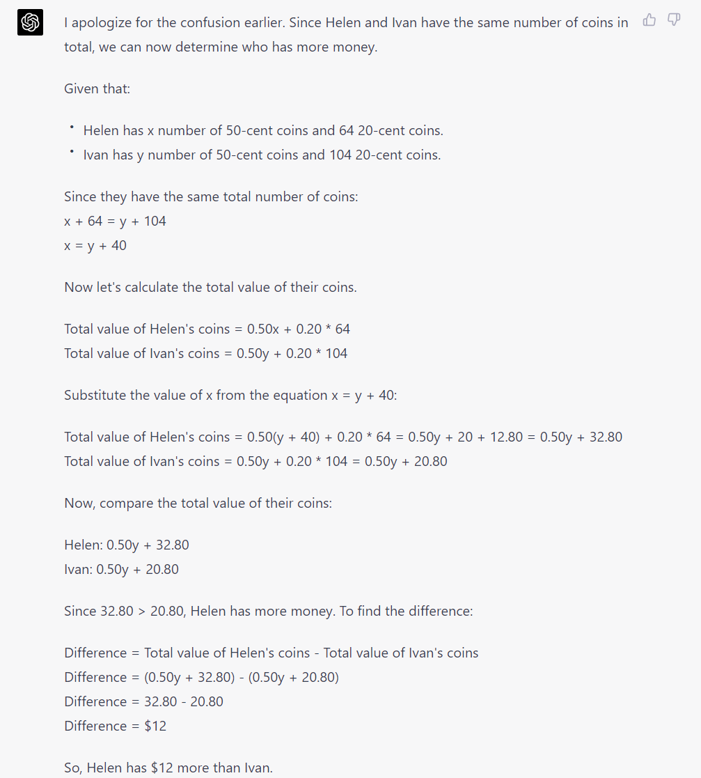
Happily, ChatGPT managed to point out the problem: it listed four possible causes, and I quickly identified the third one (lack of light source) to be the right one. ChatGPT even amended its original code to add a new light source, and lo and behold, it now worked!
Next I needed to add 27 cubes, so I asked:
How do I add 3 cubes of the same size in different parts of space?
With the reply, I could create the 27 cubes required to form a Rubik’s cube. But I recalled in many applications, one can form groups of objects for easier manipulation. So:
In WebGL, can I form a composite object comprising of three cubes?
ChatGPT suggested creating multiple THREE.Mesh objects, then putting them together in a THREE.Group object. That was exactly what I wanted.
Now to rotate a face of the cube, I needed to first identify which cubes to rotate. In each case, 9 cubes were chosen out of 27 for rotation. For that I needed the following.
In WebGL how do I access sub objects in a group object?
But ChatGPT didn’t give me what I wanted, because I had for some reason started a new conversation. The reply was ambiguous and unhelpful. So I tried again:
I have a WebGL object named “cubes” of from “THREE.Group()”. How do I access the third element in the list?
Note the grammatical mistake in the first sentence (that was completely unintentional!). Thankfully, ChatGPT correctly interpreted my intentions and gave me the following sample code (together with a rather long explanation and other variants):
let cube = cubes.children[2];
Exactly what I needed. My next thought was to put the 9 cubes in a separate group, then rotate the group. So I asked:
In WebGL, can a single cube belong to two “THREE.Group” objects simultaneously?
ChatGPT replied in the positive so I went about to edit my code, adding the 9 cubes to a separate group for rotation. But then I faced a problem:
In the following WebGL code:
function move1(all_cubes) {
var cube_list = all_cubes.children;
var tmp_group = new THREE.Group();
for(var i = 0; i < cube_list.length; i++) {
console.log(cube_list[i].position);
if (cube_list[i].position.x < -0.99)
tmp_group.add(cube_list[i]);
}
}
The object “cube_list” had some of its objects removed, when I added them to the object “tmp_group”. Why?
ChatGPT explained that the objects were being removed from the all_cubes group because they were being added to the tmp_group group. I could overcome this by cloning the cube. Finding this too much a chore, I decided against this and just rotated the 9 cubes manually. Next:
How do I rotate a 3D WebGL object with centre of rotation specified by (x, y, z)?
And so on…
Summary
Thus the general outline seems clear. At each stage I had a mental image of what I wanted to do, broke down the process into specific subtasks, then queried ChatGPT for a very concrete implementation of the said subtask. Other than the above examples, I asked:
- how I could access the mouse scroller in Javascript,
- how I could do animation in WebGL (this took a few tries with different wordings, as each time, ChatGPT would reply with a different approach),
- if I could access the contents of an array produced by a function (yes, elementary question), etc.
Here are some problems I encountered.
- ChatGPT was often down due to heavy usage.
So I had to revert to Google. After one gets used to ChatGPT’s useful replies, Google’s search results seemed frustratingly irrelevant in comparison.
- The reply was sometimes truncated.
This was rare, but fortunately when it happened, the existing reply was sufficiently useful for my purpose. In any case, people have reported we could just type ‘continue’ and ChatGPT would display the remaining response. [ Warning: this does not work for code, arguably the most important case. ]
- The answer worked but it wasn’t satisfactory to me.
For instance, ChatGPT once suggested using the TWEEN library to animate face rotations, but I considered it too much of a hassle. It took a few more queries for me to coax ChatGPT into giving me a solution using ‘render()’. In retrospect, the first reply already provided me a possible approach.
- The answer was in a different context.
Sometimes ChatGPT gave a reply using a gl.* framework, but what I really wanted was the THREE.* framework. This could be solved by further specification (e.g. ‘reformulate the reply for a THREE.Cube object type’).
- The answer just plain didn’t work.
In one instance, ChatGPT gave the following output:
THREE.Quaternion().setFromRotationMatrix(rotationMatrix);

Cubes.forEach(function(cube){
   cube.applyMatrix4(rotationMatrix);
   cube.position.sub(point);
   cube.position.applyMatrix4(rotationMatrix);
   cube.position.add(point);
   cube.quaternion.multiply(rotationQuaternion);
});
which was utterly strange since it performed a rotation, then repeat the rotation about a pivot point, before performing the rotation for a third time (using quaternion representation no less). This could be fixed by simply understanding what’s going on and editing the code on your own.
Conclusion
I have no illusions about my level of proficiency in WebGL, but this experiment proves that ChatGPT lets us get to a functional level in a remarkably short time.


.
.
of order 8.


 be the projective variety defined by the homogeneous equation
  . We define maps
  as follows
 then since
  we have
  .
. is a product in the category of quasi-projective varieties.
 be a quasi-projective variety and
  be morphisms. We will define the corresponding
  as follows. For each
  , there is an open neighbourhood U of w such that
  and
and  where
where ![F_0, F_1 \in k[T_0, \ldots, T_n]](https://s0.wp.com/latex.php?latex=F_0%2C+F_1+%5Cin+k%5BT_0%2C+%5Cldots%2C+T_n%5D&bg=ffffff&fg=333333&s=0&c=20201002) are homogeneous of the same degree and either
are homogeneous of the same degree and either  or
or  has no zero in U. Same holds for
 ![G_0, G_1 \in k[T_0, \ldots, T_n]](https://s0.wp.com/latex.php?latex=G_0%2C+G_1+%5Cin+k%5BT_0%2C+%5Cldots%2C+T_n%5D&bg=ffffff&fg=333333&s=0&c=20201002) .
. by
by  . Clearly the image of f lies in V so we get a morphism
  . It is easy to see that
  and
and  . Repeating this construction over an open cover of W, we obtain our desired
  . ♦
. ♦ , the product
  exists in the category of quasi-projective varieties and is a projective variety.
 ,
, are indxed by
  with
with  and
and  .
. .
. over all
  .
.  and
and  are open (resp. closed), so is the image of
  in
in  .
. and
and  and
and  ; without loss of generality say
  .
. is open in
  there exists a homogeneous
 ![F \in k[A_0, \ldots, A_n]](https://s0.wp.com/latex.php?latex=F+%5Cin+k%5BA_0%2C+%5Cldots%2C+A_n%5D&bg=ffffff&fg=333333&s=0&c=20201002) such that
such that  . Similarly, there exists a homogeneous
 ![G \in k[B_0, \ldots, B_m]](https://s0.wp.com/latex.php?latex=G+%5Cin+k%5BB_0%2C+%5Cldots%2C+B_m%5D&bg=ffffff&fg=333333&s=0&c=20201002) such that
such that  . Then
 in V is open. ♦
 As in the
  has the cofinite topology.
 (resp.
  ).
). are closed (resp. locally closed), so is the image W of
  and
and  then restrict to
  and
and  .
. is the product of
  in the category of quasi-projective varieties.
 ,
,  are any morphisms then
  and
and  induce
  ; the image of f lies in W so we obtain an induced
  . ♦
. ♦ be the set of points
  satisfying
  . Find a set of homogeneous polynomials in
  which define the image of W.
 is closed if and only if its corresponding subset
  is the set of solutions of some bihomogeneous polynomials
 ,
, as well as
  .
.  in a quasi-projective variety V, there is an open neighbourhood U,
  , which is affine.
 is a locally closed subset. Without loss of generality,
  so
so  , a locally closed subset of
  . Now W is open in
  , its closure in
 ![\{D(f) : f\in k[\overline W]\}](https://s0.wp.com/latex.php?latex=%5C%7BD%28f%29+%3A+f%5Cin+k%5B%5Coverline+W%5D%5C%7D&bg=ffffff&fg=333333&s=0&c=20201002) , where
, where
![f\in k[\overline W]](https://s0.wp.com/latex.php?latex=f%5Cin+k%5B%5Coverline+W%5D&bg=ffffff&fg=333333&s=0&c=20201002) we have
we have  . Now we are done since
  is isomorphic to the affine variety with coordinate ring
 ![k[\overline W][T]/(T\cdot f - 1)](https://s0.wp.com/latex.php?latex=k%5B%5Coverline+W%5D%5BT%5D%2F%28T%5Ccdot+f+-+1%29&bg=ffffff&fg=333333&s=0&c=20201002) . ♦
. ♦ is also irreducible. Again, please be reminded that
  .
. and
and  . Then
  is an open affine subset of the quasi-projective variety
  .
. be a non-empty closed subset. Then
  .
. ; by
; by  and V’ is a closed subset of
  . Now there is an isomorphism
 . ♦
. ♦ , we have
 has height 1. Pick
  such that
  has annihilator
  , i.e.
  . Since bA is finitely generated, we localize both sides at
  to obtain
  , the unique maximal ideal of
  . Thus
 . We claim that
  ; if not,
  and by the adjugate matrix trick (see
  is integral over B. This contradicts the fact that B is normal. Hence
  is an invertible ideal so B is a dvr, and
  . ♦
. ♦ , we have
  . Then
 ,
, .
. , where
  ,
,  ; we need to show
  . Write
  for its
  all of height 1. For each i we have
  . But
. But  since all
  are minimal in
  . Thus
 . ♦
. ♦![A = k[V]](https://s0.wp.com/latex.php?latex=A+%3D+k%5BV%5D&bg=ffffff&fg=333333&s=0&c=20201002) for an irreducible affine variety V, and
for an irreducible affine variety V, and  be a prime ideal with corresponding subvariety
  . Prove that
  is the set of all
  holds for all domains; geometrically, this means if
  (for irreducible V) is regular at each point, then f can be represented by the same polynomial globally. The condition in lemma 2 is notably stronger; geometrically, it says if f is regular on an open dense subset of every codimension 1 subvariety, then it is regular everywhere.
 is normal if and only if the following conditions both hold.
 .
.![k[V]](https://s0.wp.com/latex.php?latex=k%5BV%5D&bg=ffffff&fg=333333&s=0&c=20201002) is a normal domain.
is a normal domain. is a non-empty closed subset, corresponding to radical ideal
 ![\mathfrak a \subsetneq k[V]](https://s0.wp.com/latex.php?latex=%5Cmathfrak+a+%5Csubsetneq+k%5BV%5D&bg=ffffff&fg=333333&s=0&c=20201002) , the codimension of W in V is
, the codimension of W in V is  .
. is a non-empty closed subset of codimension at least 2, then the inclusion
  induces an isomorphism of coordinate rings
![k[V-W] \cong k[V]](https://s0.wp.com/latex.php?latex=k%5BV-W%5D+%5Ccong+k%5BV%5D&bg=ffffff&fg=333333&s=0&c=20201002) .
.![f \in k[V-W]](https://s0.wp.com/latex.php?latex=f+%5Cin+k%5BV-W%5D&bg=ffffff&fg=333333&s=0&c=20201002) , considered as a
, considered as a ![\mathfrak p \subset k[V]](https://s0.wp.com/latex.php?latex=%5Cmathfrak+p+%5Csubset+k%5BV%5D&bg=ffffff&fg=333333&s=0&c=20201002) of height 1, f is regular on
of height 1, f is regular on  , a dense open subset of
  . Hence by exercise A,
  and by Serre’s criterion, we have
 . ♦
. ♦ are as in proposition 1, then
  is not an affine variety.
 induces an isomorphism
 ![f^* : k[V] \to k[V-W]](https://s0.wp.com/latex.php?latex=f%5E%2A+%3A+k%5BV%5D+%5Cto+k%5BV-W%5D&bg=ffffff&fg=333333&s=0&c=20201002) . If V–W were affine, f would also be an isomorphism, which is absurd since f is not surjective. ♦
. If V–W were affine, f would also be an isomorphism, which is absurd since f is not surjective. ♦
 ) is the supremum of the lengths of all such chains.
 , the Krull dimension of X is the
  .
. be a chain of irreducible closed subsets of Y. Taking their closures in X we have
 .
. is a closed irreducible subset of X. Furthermore by a general result in point-set topology (see
  in Y is
  . Hence
  so
so  for any i. Thus we get a chain of irreducible closed subsets of X of length k. ♦
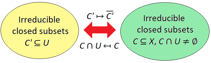
 is the closure of C’ in X.
 is a non-empty open subset of C; hence by
  .
. is an irreducible component of X.
 is an open cover for an irreducible space X, and each
  , then
  .
. . By proposition 2 we get a chain of irreducible closed subsets of
  of length k :
 .
. . ♦
. ♦ .
. .
. . Since
  is affine, by what we just showed
  . On the other hand
  by lemma 3, so equality holds throughout. ♦
 is prime if and only if:
 .
. such that
  . Since
  , among all homogeneous components of a pick
  of maximum degree such that
  ; similarly pick
  fo b so
  .
. mod
mod  , and by the given condition this means
  or
or  , a contradiction. ♦
 of a graded ring A is primary if and only if
 .
. ,
,  , where
 ![B = k[T_0, \ldots, T_n]](https://s0.wp.com/latex.php?latex=B+%3D+k%5BT_0%2C+%5Cldots%2C+T_n%5D&bg=ffffff&fg=333333&s=0&c=20201002) .
. is prime.
 . If
. If  are homogeneous, then
  and
and  are closed subsets of
  :
: .
. where
where  be closed subsets with union V. Now write
  and
and  for homogeneous radical ideals
  . Then
  . Since
  is a homogeneous radical ideal,
  . By
. By  or
or  . ♦
. ♦ is irreducible if and only if
  is irreducible.
 is prime. But
  (from an exercise
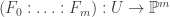
 ![F_0, \ldots, F_m \in k[T_0, \ldots, T_n]](https://s0.wp.com/latex.php?latex=F_0%2C+%5Cldots%2C+F_m+%5Cin+k%5BT_0%2C+%5Cldots%2C+T_n%5D&bg=ffffff&fg=333333&s=0&c=20201002) be homogeneous polynomials of the same degree. If
be homogeneous polynomials of the same degree. If  is such that not all
  , then we can define a function on an open subset U of
  .
. we can find an open neighbourhood U of
  . Also, if we replace projective coordinates
  with
with  , then each
  where
where  so
so
 for the resulting function.
 and
and  be quasi-projective varieties and
  be a function.
 is regular at
  if there is an open neighbourhood U of
  for some homogeneous
 ![F_i \in k[T_0, \ldots, T_n]](https://s0.wp.com/latex.php?latex=F_i+%5Cin+k%5BT_0%2C+%5Cldots%2C+T_n%5D&bg=ffffff&fg=333333&s=0&c=20201002) of the same degree.
of the same degree. , in which case we also say
  and
and  are closed subsets.
 . A regular map
  in the
  , e.g. take
  . Via embeddings
  and
and  taking
  and
and  respectively, f can be
 . This generalizes to an arbitrary regular map of closed subsets
  .
. be regular under the new definition. Then there exist polynomials
 ![f_1, \ldots, f_m \in k[X_1, \ldots, X_n]](https://s0.wp.com/latex.php?latex=f_1%2C+%5Cldots%2C+f_m+%5Cin+k%5BX_1%2C+%5Cldots%2C+X_n%5D&bg=ffffff&fg=333333&s=0&c=20201002) which represent
which represent  , let
, let  be projection onto the i-th coordinate. Then
  is regular under the new definition, and by
  can be represented as a polynomial
  . Hence we see that
 for polynomials
  given by
 works globally over the whole of
  . Let
. Let  be the closed subset defined by
  . We define a map
  as follows
 .
. .
.
 due to the equality
  since we have the reverse map
 .
. and
and  .
.![k[V] := \{ f : V\to \mathbb A^1 : f \text{ regular } \}](https://s0.wp.com/latex.php?latex=k%5BV%5D+%3A%3D+%5C%7B+f+%3A+V%5Cto+%5Cmathbb+A%5E1+%3A+f+%5Ctext%7B+regular+%7D+%5C%7D&bg=ffffff&fg=333333&s=0&c=20201002) ,
,
 of quasi-projective varieties induces a ring homomorphism
 ![\phi^* : k[W] \to k[V]](https://s0.wp.com/latex.php?latex=%5Cphi%5E%2A+%3A+k%5BW%5D+%5Cto+k%5BV%5D&bg=ffffff&fg=333333&s=0&c=20201002) . By lemma 2, when V is affine
. By lemma 2, when V is affine  , we have an automorphism
 for
for  . Also
  if and only if g is a scalar multiple of the identity matrix, so we get an injective homomorphism
  . In fact this is an isomorphism of groups.
![\left[\begin{pmatrix} a & b \\ c & d \end{pmatrix} \in GL_2 k \right] : (t_0 : t_1) \mapsto (at_0 + bt_1 : ct_0 + dt_1).](https://s0.wp.com/latex.php?latex=%5Cleft%5B%5Cbegin%7Bpmatrix%7D+a+%26+b+%5C%5C+c+%26+d+%5Cend%7Bpmatrix%7D+%5Cin+GL_2+k+%5Cright%5D+%3A+%28t_0+%3A+t_1%29+%5Cmapsto+%28at_0+%2B+bt_1+%3A+ct_0+%2B+dt_1%29.&bg=ffffff&fg=333333&s=0&c=20201002)
 and
and  via the maps
 is an affine variety even though it is not closed in
  . From the isomorphism we also have:
![k[\mathbb A^1 - \{0\}] \cong k[V] = k[X, Y]/(XY - 1) \implies k[\mathbb A^1 - \{0\}] = k[X, \frac 1 X].](https://s0.wp.com/latex.php?latex=k%5B%5Cmathbb+A%5E1+-+%5C%7B0%5C%7D%5D+%5Ccong+k%5BV%5D+%3D+k%5BX%2C+Y%5D%2F%28XY+-+1%29+%5Cimplies+k%5B%5Cmathbb+A%5E1+-+%5C%7B0%5C%7D%5D+%3D+k%5BX%2C+%5Cfrac+1+X%5D.&bg=ffffff&fg=333333&s=0&c=20201002)
 . We will show that V is not affine. Indeed consider the injection
  which induces
![\phi^* : k[X, Y] \cong k[\mathbb A^2] \longrightarrow k[V]](https://s0.wp.com/latex.php?latex=%5Cphi%5E%2A+%3A+k%5BX%2C+Y%5D+%5Ccong+k%5B%5Cmathbb+A%5E2%5D+%5Clongrightarrow+k%5BV%5D&bg=ffffff&fg=333333&s=0&c=20201002) .
. . Let us show that it is surjective. Suppose
 ![f \in k[V]](https://s0.wp.com/latex.php?latex=f+%5Cin+k%5BV%5D&bg=ffffff&fg=333333&s=0&c=20201002) so that
so that  is regular. Write
 where
where  .
.![f|_U \in k[U] \cong k[X, Y, \frac 1 X]](https://s0.wp.com/latex.php?latex=f%7C_U+%5Cin+k%5BU%5D+%5Ccong+k%5BX%2C+Y%2C+%5Cfrac+1+X%5D&bg=ffffff&fg=333333&s=0&c=20201002) and
and ![f|_{U'} \in k[U']\cong k[X, Y, \frac 1 Y]](https://s0.wp.com/latex.php?latex=f%7C_%7BU%27%7D+%5Cin+k%5BU%27%5D%5Ccong+k%5BX%2C+Y%2C+%5Cfrac+1+Y%5D&bg=ffffff&fg=333333&s=0&c=20201002) . Since
. Since  are all dense in V we have injections
 ![k[V] \to k[U] \to k[U\cap U']](https://s0.wp.com/latex.php?latex=k%5BV%5D+%5Cto+k%5BU%5D+%5Cto+k%5BU%5Ccap+U%27%5D&bg=ffffff&fg=333333&s=0&c=20201002) and
and ![k[V] \to k[U'] \to k[U\cap U']](https://s0.wp.com/latex.php?latex=k%5BV%5D+%5Cto+k%5BU%27%5D+%5Cto+k%5BU%5Ccap+U%27%5D&bg=ffffff&fg=333333&s=0&c=20201002) so that
so that ![f \in k[X, Y, \frac 1 X] \cap k[X, Y, \frac 1 Y]](https://s0.wp.com/latex.php?latex=f+%5Cin+k%5BX%2C+Y%2C+%5Cfrac+1+X%5D+%5Ccap+k%5BX%2C+Y%2C+%5Cfrac+1+Y%5D&bg=ffffff&fg=333333&s=0&c=20201002) . It is easy to show that this means
. It is easy to show that this means ![f\in k[X, Y]](https://s0.wp.com/latex.php?latex=f%5Cin+k%5BX%2C+Y%5D&bg=ffffff&fg=333333&s=0&c=20201002) .
.![k[\mathbb A^2] \to k[V]](https://s0.wp.com/latex.php?latex=k%5B%5Cmathbb+A%5E2%5D+%5Cto+k%5BV%5D&bg=ffffff&fg=333333&s=0&c=20201002) . If V is affine, by
. If V is affine, by  . On the set
  , we consider the equivalence relation:
 for any representative
  .
. .
. is homogeneous and
  . We write
  if
if  .
. is in general not well-defined. Indeed if we have two representatives
  for
for 
 if and only if
  be a
be a  .
. we also write
  for
for  where
where  .
. .
. and collection of graded ideals
  of B.
of B. .
. is a set of homogeneous generators of
  .
. .
. .
. .
.

 the same point can be represented by
  where the i-th coordinate is 1. This gives a bijection
  . E.g. for n = 2, we have:
 , the intersection
  maps to an open subset of
  and
and  . Indeed if i < j then
  is the set of all
  satisfying
  while
while  is the set of all
  . Hence, the following is well-defined.
 as an open subset, where
  .
. , the set
  is (Zariski) closed in
  is closed in
  . But
. But  , where
 ![f(X_1, \ldots, X_n) = F(1, X_1, \ldots, X_n) \in k[X_1, \ldots, X_n]](https://s0.wp.com/latex.php?latex=f%28X_1%2C+%5Cldots%2C+X_n%29+%3D+F%281%2C+X_1%2C+%5Cldots%2C+X_n%29+%5Cin+k%5BX_1%2C+%5Cldots%2C+X_n%5D&bg=ffffff&fg=333333&s=0&c=20201002) . The same holds for
. The same holds for  . ♦
. ♦![f \in k[X_1, \ldots, X_n]](https://s0.wp.com/latex.php?latex=f+%5Cin+k%5BX_1%2C+%5Cldots%2C+X_n%5D&bg=ffffff&fg=333333&s=0&c=20201002) , let
, let
![f,g\in k[X_1, \ldots, X_n]](https://s0.wp.com/latex.php?latex=f%2Cg%5Cin+k%5BX_1%2C+%5Cldots%2C+X_n%5D&bg=ffffff&fg=333333&s=0&c=20201002) , the homogenization of fg is the product of the homogenizations of f and g.
, the homogenization of fg is the product of the homogenizations of f and g.![F\in k[T_0, \ldots, T_n]](https://s0.wp.com/latex.php?latex=F%5Cin+k%5BT_0%2C+%5Cldots%2C+T_n%5D&bg=ffffff&fg=333333&s=0&c=20201002) be the homogenization of a non-constant
be the homogenization of a non-constant  for some graded ideal
  . Since
  , by lemma 1 this is Zariski closed.
 ; it suffices to show that any
  is contained in
  for some homogeneous
  without loss of generality. Hence
  for some
  , then
 , where F = homogenization of f. ♦
 be the projective variety defined by the homogeneous equation
  . Then
 is cut out from
  by
by  ;
; is cut out from
  ;
; is cut out from
  .
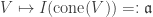
. be any subset. The cone of C is
 .
. we have
 is a proper graded ideal then
  .
. is closed in
  .
. . Now pick a set of homogeneous generators
  for
for  .
. is of the form
  .
. .
. . Let
. Let  so that
  . It remains to show
  by lemma 2.
 , write
  as a sum of homogeneous components. Then for any
  and
and  we have
  which gives
 vanish for any
  . ♦
. ♦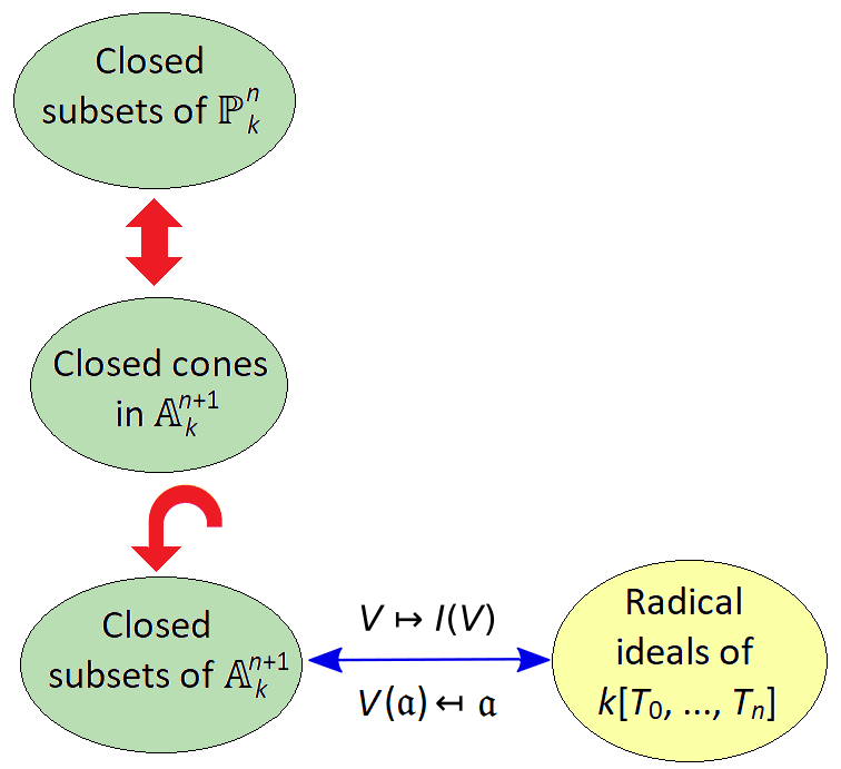
 , the ideal
  is graded. Conversely, if
 ![\mathfrak a\subsetneq k[T_0, \ldots, T_n]](https://s0.wp.com/latex.php?latex=%5Cmathfrak+a%5Csubsetneq+k%5BT_0%2C+%5Cldots%2C+T_n%5D&bg=ffffff&fg=333333&s=0&c=20201002) is graded,
is graded,  is the (non-empty) solution set of a collection of graded polynomials; hence it is a closed cone too.
![\mathfrak a \subsetneq B = k[T_0, \ldots, T_n]](https://s0.wp.com/latex.php?latex=%5Cmathfrak+a+%5Csubsetneq+B+%3D+k%5BT_0%2C+%5Cldots%2C+T_n%5D&bg=ffffff&fg=333333&s=0&c=20201002) .
. and so
 which takes closed subsets of
  .
. so we modify our bijection to:
 is the irrelevant ideal of B.
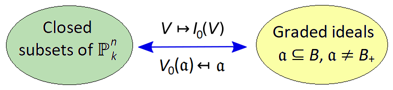
 .
. be a proper ideal. A primary decomposition of
 is
is  , i.e.
  .
. is
is  ,
, .
. is the
  . By
. By  is
is  and
and  , then
  is a zero-divisor of
  .
. , suppose
  ; then
  is a zero-divisor for
  and we have
  . Conversely, if
  is an associated prime of
  .
. and
and  . For some n > 0,
  . But
. But  so by the given condition
  and
and  .
. . First,
  .
. and
and  are such that
  , then by the given condition
  . ♦
. ♦ is primary if:
 .
. is a ring homomorphism and
  is a primary ideal, then
  is a primary ideal of A. Also
  .
. , there is a bijection between primary ideals of A containing
  .
. is a fixed multiplicative subset.
 such that
  ;
;
 , then
 .
. is primary and
  is primary, and
 .
. is a proper ideal since
  satisfy
  ; then for some
  we have
  . Since
  .
. . Conversely let
  satisfy
  . For some
  we have
  . As above
  so
so  . ♦
. ♦
 for each i. If
  .
. at
at  . But since
  .
. . By proposition 2 this gives
  which is uniquely determined by
  is maximal, then
  for some n > 0.
![A =k[X, Y, Z]/(Z^2 - XY)](https://s0.wp.com/latex.php?latex=A+%3Dk%5BX%2C+Y%2C+Z%5D%2F%28Z%5E2+-+XY%29&bg=ffffff&fg=333333&s=0&c=20201002) with
with  , which is prime since
![A/\mathfrak p \cong k[X, Y, Z]/(Z^2 - XY, X, Z) \cong k[Y]](https://s0.wp.com/latex.php?latex=A%2F%5Cmathfrak+p+%5Ccong+k%5BX%2C+Y%2C+Z%5D%2F%28Z%5E2+-+XY%2C+X%2C+Z%29+%5Ccong+k%5BY%5D&bg=ffffff&fg=333333&s=0&c=20201002) .
. is not primary because
  but
but  and
and  .
.![A = k[X, Y]](https://s0.wp.com/latex.php?latex=A+%3D+k%5BX%2C+Y%5D&bg=ffffff&fg=333333&s=0&c=20201002) and
and  , the A-module
  .
. is prime and hence primary;
 is a power of the maximal ideal
  ; by exercise B.2 it is primary;
 so
so  is primary by exercise B.2.
 . Geometrically, the k-scheme with coordinate ring
![A = k[X, Y, Z]](https://s0.wp.com/latex.php?latex=A+%3D+k%5BX%2C+Y%2C+Z%5D&bg=ffffff&fg=333333&s=0&c=20201002) with
with  . Then
![k[X, Y, Z]/(X - YZ) \cong k[Y, Z], \ X \mapsto YZ \implies k[X, Y, Z]/\mathfrak a \cong k[Y, Z]/(Y^2 Z)](https://s0.wp.com/latex.php?latex=k%5BX%2C+Y%2C+Z%5D%2F%28X+-+YZ%29+%5Ccong+k%5BY%2C+Z%5D%2C+%5C+X+%5Cmapsto+YZ+%5Cimplies+k%5BX%2C+Y%2C+Z%5D%2F%5Cmathfrak+a+%5Ccong+k%5BY%2C+Z%5D%2F%28Y%5E2+Z%29&bg=ffffff&fg=333333&s=0&c=20201002) .
. , an intersection of primary ideals with
  and
and  . This translates to
 and
and  is already prime.
 . Then each of
  and
and  is primary (the first ideal is prime; the remaining two ideals are powers of a maximal ideal). Hence this gives a primary decomposition of
  , with the latter two embedded.
 ,
,  ,
,  be ideals of A. Set
  . Prove that

 as A-modules for prime ideals
  .
. . Since
  by
by  . If equality holds, we are done. Otherwise, let
  be the image of the map and repeat with
  to obtain a submodule
  . Repeating this process, this must eventually terminate since we cannot have an infinite ascending chain of submodules
  . ♦
. ♦ be as in proposition 1 with
  for some prime
  .
. is finite.
 for each i, we are done. ♦
 , then there is a map
  and so
  . Hence we have shown:
 .
. then
then  .
.
 ; but since
  so
so
![M = k[X, Y]/(X^2, XY)](https://s0.wp.com/latex.php?latex=M+%3D+k%5BX%2C+Y%5D%2F%28X%5E2%2C+XY%29&bg=ffffff&fg=333333&s=0&c=20201002) , considered as an A-module. Note that
, considered as an A-module. Note that  with radical
  .
. . Indeed we have:
 and
and  with
with  . Then
  ; as shown above,
  . Also
  so by corollary 1
 .
. with
with  but
but  .
. of all submodules
  such that
  . Note that
 .
. .
. .
. then
then  so the above intersection only needs to be taken over
  . If
. If  it has an associated prime
  we have
  , a contradiction. ♦
 .
. . Since
  we have
  . On the other hand if
  , then we have an injection
  whose image is of the form
  . But now
 . Hence no such
  .
.
 is a
is a  ,
,  . It is minimal if it is irredundant and all
  ,
,  must be a maximal element of
  are
are  .
. the canonical map
  is injective. Hence
 ♦
♦ then among the injections
  and
and  , we have
  since
since  are disjoint. Thus
 is injective
 , contradicting the condition of irredundancy. ♦
 to be distinct.

 is a
is a  , every non-zero ideal is an intersection of
  , ideals generated by prime powers.
 in A is
 ,
, ,
, , we say M is a faithful A-module.
 , then M can be regarded as a faithful
  , let
, let .
.
 in terms of annihilators.
 if P is a finitely generated submodule of M.
 .
.

 .
. we have
  is zero if and only if there exists
  such that
  , equivalently if there exists
  . Hence
  if and only if
  .
. generate M as an A-module. Then
 if and only if it contains either
  is a short exact sequence of A-modules, then
  .
. .
. if and only if both terms are zero whereas
  if and only if at least one term is zero.
 and it follows that
  if and only if
  .
.
 or
or  , clearly the RHS is zero. Conversely if both are non-zero, since they are finitely generated
  and
and  . But these are vector spaces over
  so we have
![k(\mathfrak p) \otimes_A N \otimes_A P = [k(\mathfrak p) \otimes_A N] \otimes_{k(\mathfrak p)} [k(\mathfrak p) \otimes_A P] \ne 0 \implies (N\otimes_A P)_{\mathfrak p} \ne 0.](https://s0.wp.com/latex.php?latex=k%28%5Cmathfrak+p%29+%5Cotimes_A+N+%5Cotimes_A+P+%3D+%5Bk%28%5Cmathfrak+p%29+%5Cotimes_A+N%5D+%5Cotimes_%7Bk%28%5Cmathfrak+p%29%7D+%5Bk%28%5Cmathfrak+p%29+%5Cotimes_A+P%5D+%5Cne+0+%5Cimplies+%28N%5Cotimes_A+P%29_%7B%5Cmathfrak+p%7D+%5Cne+0.&bg=ffffff&fg=333333&s=0&c=20201002) ♦
♦ be a homomorphism of finitely generated A-modules; prove that
  is a closed subset of Spec A.
 for some
  is
is  . There is a bijection
 .
. by considering
  .
. such that
  ; we need to show a is contained in an associated prime of M.
 be the set of ideals of A containing a of the form
  for
for  . Since A is noetherian and
  , there is a maximal
  . We will show
  for some
  .
. such that
  and
and  . Since
  , we have
  . And since
  , by maximality of
  we have
  . ♦
. ♦ be a short exact sequence of A-modules. Then
 . The first containment in the claim is obvious. For the second, suppose we have an A-linear map
  .
. , then any non-zero
  has annihilator
  . If
. If  , then composing
  is still injective, so
  . ♦
. ♦ .
.
 , then localization at S gives an A-linear map
  .
. -linear map
  where
where  is prime. By
  for some prime
  we let
  be the image of 1. It remains to show: there exists
  such that
  .
. , we have
  in
in  so that
  in M for some
  . Pick a generating set
  of
of  with
with  . Then
  satisfies
  .
. then
then  so
so  lies in the annihilator of
  ; since