
The Hom Group
Continuing from the previous installation, here’s another way of writing the universal properties for direct sums and products. Let Hom(M, N) be the set of all module homomorphisms M → N; then:

for any R-module N.
In the case where there’re finitely many Mi‘s, the direct product and direct sum are identical, so we get:

This correspondence is extremely important. One can write this as a matrix form: 


In fact, there’s more to the correspondence (**) than a mere bijection of sets:
Proposition. The set Hom(M, N) forms an abelian group; if
are module homomorphisms, then we define:
The identity is given by f(m) = 0 for all m; it is also denoted by


Since the proof is straightforward, we’ll leave it as a simple exercise. The bijections in (*) and (**) are thus isomorphisms of abelian groups.

Free Modules
First we define:
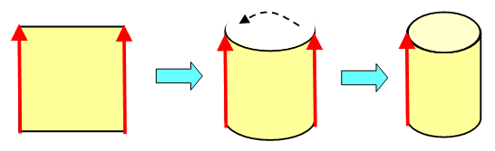
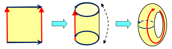
Definition. Let I be an index set. The free module on I is the direct sum of copies of R, indexed by elements of I:
In contrast, the direct product of copies of R is given by
.
You might wonder why we’re interested in direct sum and not the product; it’s because of its universal property.
From the correspondence in (*), we obtain:

On the other hand, it’s easy to see that 


In fact, we can say this is an isomorphism of R-modules, if we define an R-module structure on Hom(R, M) by letting 


Thus, we get:

where the RHS is a direct product. Thus, the free module satisfies the following universal property:
Universal Property of Free Modules. There is a 1-1 correspondence between module homomorphisms
and elements of the direct product

Rank of Free Modules
Finite free modules (i.e. free modules 

Composition of linear maps 

Question. If
, then we call #I the rank of M. Is the rank well-defined? E.g. is it possible for
to occur as R-modules?
This turns out to be a rather difficult problem, since the answer is (no, yes), when phrased in the most general setting. In other words, there exist rings R for which 


- Division rings (and hence fields) satisfy IBN.
- Non-trivial commutative rings satisfy IBN.
The second case follows from the first if we’re allowed to use a standard result in commutative algebra: every non-trivial commutative ring R ≠ 1 has a maximal ideal I. Assuming this, if 


The case of division rings will be proven later.
Basis of Free Module
Free modules are probably the most well-behaved types of modules since many of the results in standard linear algebra carry over, e.g. the presence of a basis.
Definition. A subset S of module M is said to be linearly independent if whenever
and
satisfy:
,
we have
.
Definition. A subset S of M is said to be a basis if it is linearly independent and generates the module M.
Clearly, a subset of a linearly independent set is linearly independent as well. On the other hand, a superset of a generating set also generates the module. Thus, the basis lies as a fine balance between the two cases.
A free module 


For example, if I = {1, 2, 3}, the standard basis is given by

which is hardly surprising if you’ve done linear algebra before.
Conversely, any module with a basis is free.
Proposition. If
is a basis, with elements indexed by
, then there’s an isomorphism:
, which takes

Sketch of Proof.
First note that the RHS sum is well-defined since there’re only finitely many non-zero terms for ri. The map is also clearly R-linear. The fact that it’s surjective is precisely the condition that the mi‘s generate M. Also it’s injective if and only if the kernel is 0, which is exactly the condition that S is linearly independent. ♦
In conclusion:
Corollary. An R-module is free if and only if it has a basis.
Clearly, not all R-modules have a basis. This is amply clear even for the case R=Z, since the finite Z-module (i.e. abelian group) Z/2 has no basis. On the other hand, for R=Z, every submodule of a free module is free. This does not hold for a general ring, e.g. for R = R[x, y], the ring of polynomials in x, y with real coefficients, the ideal <x, y> is a submodule which is not free since any two elements are linearly dependent.
Finally, the astute reader who had any exposure to linear algebra would not be surprised to see the following.
Theorem. Every module over a division ring has a basis, and the cardinality of the basis (i.e. the rank of the module) is well-defined.
Question.
Let 
Linear Algebra Over Division Rings.
Let R be a division ring D for the remaining of this article. A D-module will henceforth be known as a vector space over D, in accordance with linear algebra.
Theorem (Existence of Basis). Every vector space over D has a basis. Specifically, if
are subsets such that S is linearly independent and T is a generating set, then there’s a basis B such that
[ In particular, any linearly independent subset can be extended to a basis and any generating set has a subset which is a basis. ]

This gist of the proof is to keep adding elements to S while keeping it linearly independent, until one can’t add anymore. This will result in a basis.
Proof.
First, establish the groundwork for Zorn’s lemma.
- Let Σ be the class of all linearly independent sets U where
Now Σ is not empty since
at least.
- Partially order Σ by inclusion.
- If
is a chain (i.e. for any a, b we have
or
), then the union
is also linearly independent and
- Indeed, U is linearly independent because any linear dependency
would involve only finitely many terms
, so all these terms would come from a single Ua, thus violating its linear independence.
- Indeed, U is linearly independent because any linear dependency
Hence, Zorn’s lemma tells us there’s a maximal linearly independent U among all 


which is a contradiction. Hence, U’ is a linearly independent set strictly containing U and contained in T, which violates the maximality of U. Conclusion: U is a basis. ♦
Theorem (Uniqueness of Rank). If
, then I and J have the same cardinality.
The gist of the proof is to replace elements of one basis with another, and show that there’s an injection I → J.
Proof.
Let 

- Take the class Σ of all injections
such that
is a basis of M.
- Now Σ is not empty since it contains
.
- Partially order Σ as follows: (φ: S → J) ≤ (φ’: S’ → J) if and only if
and
- Show that if
is a chain in Σ, then one can take the “union”
where
for any a such that


Hence, Zorn’s lemma applies and there’s a maximal 

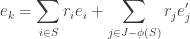

Since the ei‘s are linearly independent, the second sum is non-empty so pick any j’ for which 

Hence, we can extend 
The dimension of a vector space over a division ring is thus defined to be the cardinality of any basis. It is a well-defined value.


 be the ring of n × n matrices with integer entries. Then
  is a module and
  is a submodule. The resulting quotient is isomorphic to
 be an ideal of R and M be an R-module. The module quotient M/IM is not only an R-module, but an (R/I)-module as well. Indeed, if
  then multiplying with
  gives
gives  This is well-defined since if
  and
and  , then we have
  and
and  which gives us
  and so rm + I = r’m’ + I. Thus scalar multiplication by R/I is well-defined and it’s easy to show that M/IM is an R/I-module.
 and
and 
 and
and  be a homomorphism of R-modules.
 is a submodule, then f(M’) is a submodule of N.
 is a submodule, then f-1(N’) is a submodule of M.
 and
and  and
and  and we’re done. ♦
 , the pullback
  is called the kernel of f; this is a submodule of M, denoted ker(f).
 is called the image of f; this is a submodule of N, denoted im(f).
 .
.
 which takes
  to f(m). Let’s show that g is injective and well-defined. Indeed:

 be submodules. Then N/P is a submodule of M/P and
 with projection
  Apply the first isomorphism theorem. The kernel of this map is
  while the image is the whole of (N+N’)/N’ since any element (n+n’)+N’ (for
  and
and  ) is basically just n+N’.
 . As in the case of groups and rings, there’s a correspondence between submodules of M containing N, as well as submodules of M/N.

 always holds, and that if P contains N, then we have
  . ♦
. ♦ .
. . It’s given the structure of an R-module, by letting
  is the subset of
  for which only finitely many mi‘s are non-zero. This is clearly a submodule of the direct product.
 be the projection map. If N is a module and
  is any collection of module homomorphisms, then there’s a unique
  such that:
 for all j.
 be the natural inclusion map which takes
  to the tuple
  which comprises of all zeros except
  If N is a module and
  is any collection of module homomorphisms, then there’s a unique
  such that:
 for all j.
 for all
  for any
 . Explain why
  ) such that for any
  and
and  we have:
 ;
; ;
; ;
; .
. is often called scalar multiplication, since one should think of elements of M as “vectors” and those of R as “scalars”, following the terminology of linear algebra.
 , where
  and
and  ;
; . Adding
  to both sides gives
  The other equality is left as an easy exercise.
 and
and  in which case one can turn a right R-module into a left one via this isomorphism. For example, if H denotes the division ring of all quaternions with real coefficients, then:
 where * is the product operation for the opposite ring.
 and gives us the structure of a Z-module).
 is an R-module, where scalar multiplication is given by ring product in R.
 , the Cartesian product of n copies of R. Product is given by
 be the ring of matrices with integer entries. Then
  is an R-module, via multiplying a matrix by vector.
 ;
; then
then  ;
; , then
  .
. m–n = m+(-1)n also lies in N. Thus, we can replace the first condition with
  since we can then pick
  from the second and third conditions.
 is a collection of submodules of M, then
  is a submodule of M;and
 is the set of all sums of finitely many terms from
 , then
  for every i. Hence,
  for every i, which gives
  Finally, suppose
  for each i so
  for each i. Hence
 and clearly N’ is closed under addition since if
  are sums of finitely many terms from
  , then x+y is obtained by concatenating the two sums. Finally
  where each
  ♦
♦ be any subset and consider:
 : indeed, it’s an intersection of N‘s, each of which contains S.
 , then
  : indeed since N’ contains S, it’s found in the collection ∑. Since <S> is defined to be the intersection of N’ and some other submodules, we have
 Indeed, since
  we clearly have
  for any scalar
  On the other hand, it’s easy to check that Rm is itself a submodule of M containing m. Hence,
  and the two sets are equal.
 ;
; , then
  ;
; , then
  .
.
 where
where  and
and 
 Then
Then  is a proper submodule of M.
 of n × n real matrices and module
  one sees that there’s no proper submodule. In other words, any single non-zero
  generates the whole module M. Such modules are called simple modules and we’ll encounter them again later.
 . First, we have the trivial and alternating representations (see
  maps to a permutation matrix, the trace is precisely the number of fixed points. This gives:
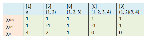
 so
so  contains 1 copy of the trivial representation. And since
  it doesn’t include the alternating representation. Subtracting gives:
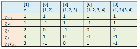
 so we’ve found another irreducible representation. Tensor product gives
  which is also easily checked to be irreducible. Since we’ve found 4 out of 5 irreducible representations, the remaining one is easy. First, the degree must be
  so the regular representation must contain two copies of it. This gives:
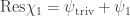
 as well. As before, we have the trivial and alternating representations. Again, the natural action of G on {1, 2, 3, 4, 5} gives:
 and
and  One easily checks that
  which is easily checked to be irreducible as well.
 is a rather huge representation (of degree 16), so let’s take a subspace instead.
 . The swapping map
  which takes
  is clearly bilinear, so it induces a linear map
  which takes
  Clearly f2 is the identity, since it maps all elements of the form
  back to themselves and the set of all such elements spans
  Since a power of f is the identity, f is diagonalisable. Its eigenvalues must satisfy
  so:
so:
 and
and  respectively. Clearly, if
  is a basis of V, then a basis of
  (resp.
  ).
). and
and  respectively.
 is invariant under every
  To prove this, it suffices to show g commutes with the swapping map above
  This fact isn’t hard to prove:
 . Since f commutes with g, a standard result from linear algebra tells us g is invariant on the eigenspaces of f. Thus
  and
and 
 in terms of
  .
. then we have:
 . Since
  and
and  it follows that:
 above, then:
 and
and 
 is irreducible. On the other hand
  and
and  so taking the difference gives the sixth irreducible character:
 . Conclusion:
 . Since this is a subgroup of S5, let’s take the above 7 characters and restrict them to
  However, we’re now left with only 4 since 3 of the characters are paired via
  such that
  (we say that the two characters are twists of each other).
 so it’s a direct sum of two non-isomorphic irreducible representations. Since
  and
and  so
so 

 to obtain some orthonormal basis:
 , where
  and
and  .
. is one of the last two irreducible characters, then we can write
  for real values a, b satisfying
  Since
Since  we also have
  which gives:
 or
or  and our work is done.
 to that of H. We’ll denote this restricted representation by
  and the corresponding character

 is irreducible, its restriction to H may not be. Even worse, even if
 and
and  are orthogonal (i.e.
  ), their restrictions to H may not be. We’ll see this in an example later on.
 , we’ll define an induced representation (denoted
  and
and  ). Abstractly, if V is a C[H]-module, we take:
![W := \mathbf{C}[G]\otimes_{\mathbf{C}[H]} V](https://s0.wp.com/latex.php?latex=W+%3A%3D+%5Cmathbf%7BC%7D%5BG%5D%5Cotimes_%7B%5Cmathbf%7BC%7D%5BH%5D%7D+V&bg=ffffff&fg=333333&s=0&c=20201002)
 – this follows from the more general fact that if
  are rings, then
  is functorial. The case for Res is obvious. Furthermore, we have:
 and
and 
 are rings, then there’s a natural isomorphism
  for any R-module M. ♦
![R = \mathbf{C}[H]](https://s0.wp.com/latex.php?latex=R+%3D+%5Cmathbf%7BC%7D%5BH%5D&bg=ffffff&fg=333333&s=0&c=20201002) and
and ![S = \mathbf{C}[G]](https://s0.wp.com/latex.php?latex=S+%3D+%5Cmathbf%7BC%7D%5BG%5D&bg=ffffff&fg=333333&s=0&c=20201002) and let the characters for M and N be denoted by
and let the characters for M and N be denoted by  and
and ![\begin{aligned}LHS:& \dim_\mathbf{C} \text{Hom}_{\mathbf{C}[G]}(\mathbf{C}[G]\otimes_{\mathbf{C}[H]} M, N) = \left<\text{Ind}_H^G \psi, \chi\right>_G,\\ RHS:& \dim_\mathbf{C} \text{Hom}_{\mathbf{C}[H]} (M, N)= \left<\psi, \text{Res}_G^H \chi\right>_H.\end{aligned}](https://s0.wp.com/latex.php?latex=%5Cbegin%7Baligned%7DLHS%3A%26+%5Cdim_%5Cmathbf%7BC%7D+%5Ctext%7BHom%7D_%7B%5Cmathbf%7BC%7D%5BG%5D%7D%28%5Cmathbf%7BC%7D%5BG%5D%5Cotimes_%7B%5Cmathbf%7BC%7D%5BH%5D%7D+M%2C+N%29+%3D+%5Cleft%3C%5Ctext%7BInd%7D_H%5EG+%5Cpsi%2C+%5Cchi%5Cright%3E_G%2C%5C%5C+RHS%3A%26+%5Cdim_%5Cmathbf%7BC%7D+%5Ctext%7BHom%7D_%7B%5Cmathbf%7BC%7D%5BH%5D%7D+%28M%2C+N%29%3D+%5Cleft%3C%5Cpsi%2C+%5Ctext%7BRes%7D_G%5EH+%5Cchi%5Cright%3E_H.%5Cend%7Baligned%7D&bg=ffffff&fg=333333&s=0&c=20201002)
 are characters of representations, then:
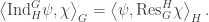
 and
and 
 Their character tables are given below:
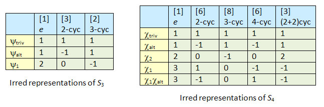
 ;
; ;
; ;
; ;
; .
.
 ,
, where the gi‘s is a set of left coset representatives for G/H. Hence if M is a C[H]-module, then
 ![M' :=\mathbf{C}[G]\otimes_{\mathbf{C}[H]} M](https://s0.wp.com/latex.php?latex=M%27+%3A%3D%5Cmathbf%7BC%7D%5BG%5D%5Cotimes_%7B%5Cmathbf%7BC%7D%5BH%5D%7D+M&bg=ffffff&fg=333333&s=0&c=20201002) is the direct sum of
is the direct sum of  where M is identified with
 around; if
  then there’s no contribution from
  so the contribution to the trace is exactly
  i.e.
i.e.
 ; it turns out to be much more convenient to apply the first equality above:
  For coset representatives of
  let us take
  for i = 0, 1, 2, 3:
 for each i. Thus
 only for i=0, 3. Thus

 so
so 


 and
and  . [ Hint: to compute the character table of A4, pick the normal subgroup
  and consider the character table of A4/N. ]
![\alpha = \sum_{g\in G} f(g)g\in \mathbf{C}[G].](https://s0.wp.com/latex.php?latex=%5Calpha+%3D+%5Csum_%7Bg%5Cin+G%7D+f%28g%29g%5Cin+%5Cmathbf%7BC%7D%5BG%5D.&bg=ffffff&fg=333333&s=0&c=20201002)
 , take the element
 ![e_C := \sum_{g\in C} g\in \mathbf{C}[G].](https://s0.wp.com/latex.php?latex=e_C+%3A%3D+%5Csum_%7Bg%5Cin+C%7D+g%5Cin+%5Cmathbf%7BC%7D%5BG%5D.&bg=ffffff&fg=333333&s=0&c=20201002)
 commutes with anything in C[G].
![e_C\in \mathbf{Z}[G]](https://s0.wp.com/latex.php?latex=e_C%5Cin+%5Cmathbf%7BZ%7D%5BG%5D&bg=ffffff&fg=333333&s=0&c=20201002) and Z[G] is a ring which is a finite Z-module,
and Z[G] is a ring which is a finite Z-module,  is a linear combination of
  with coefficients which are algebraic integers. Thus, α is a sum of commuting elements, each of which is integral over Z. Conclusion: α satisfies a monic polynomial with integer coefficients.
![\alpha g = g\alpha\in \mathbf{C}[G]](https://s0.wp.com/latex.php?latex=%5Calpha+g+%3D+g%5Calpha%5Cin+%5Cmathbf%7BC%7D%5BG%5D&bg=ffffff&fg=333333&s=0&c=20201002) for any
for any 
 ; each f(g) is an algebraic integer since the eigenvalues of g are roots of unity and thus algebraic integers. Now
  by orthonormality of irreducible characters. Thus
  is an algebraic integer which lies in Q, so it’s an integer. ♦
 is a K[G]-submodule, it turns out V is isomorphic to the direct sum of W and some other submodule W’.
 such that:
 .
. ; since V is finite-dimensional, this process must eventually terminate.
 and
and  , which is always possible by linear algebra. Take the projection map
  Now define the linear map:
 But
But
 then q(w)=w. Indeed since W is a K[G]-submodule of V,
  so
so  for every
  , then q(v) = 0 since
  on the other hand, since
  we have q(v)=v so v=0. Thus,
 , write
  . Since
  we have
  also. So
  and we get
  Thus
Thus  ♦
♦ acting on
  by permuting the coordinates (see
![\dim_{\mathbf{C}} \text{Hom}_{\mathbf{C}[G]}(V, W) = \begin{cases} 0, \quad &\text{if } V\not\cong W,\\ 1,\quad &\text{if } V\cong W.\end{cases}](https://s0.wp.com/latex.php?latex=%5Cdim_%7B%5Cmathbf%7BC%7D%7D+%5Ctext%7BHom%7D_%7B%5Cmathbf%7BC%7D%5BG%5D%7D%28V%2C+W%29+%3D+%5Cbegin%7Bcases%7D+0%2C+%5Cquad+%26%5Ctext%7Bif+%7D+V%5Cnot%5Ccong+W%2C%5C%5C+1%2C%5Cquad+%26%5Ctext%7Bif+%7D+V%5Ccong+W.%5Cend%7Bcases%7D&bg=ffffff&fg=333333&s=0&c=20201002)


 . Indeed, for any
  , we have
 then gw = w, which gives us p(w) = w. Just as in the proof of Maschke’s theorem, this shows
  and
and 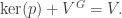 If we pick a basis of ker(p) and of VG, then the matrix for p is:
 ♦
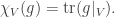
♦ be a representation of G. Its character is the function
 Suppose V and W are C[G]-modules. Let’s consider the various constructions in G3.
 .
. .
. .
. of V and consider the dual basis
  If M is the matrix for g : V → V with respect to B, the corresponding matrix for g : V* → V* with respect to B* is given by
  Hence:
 Thus g-1 is diagonal with entries
  and
and  as desired.

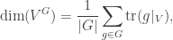
![\text{Hom}_{\mathbf{C}}(V, W)^G = \text{Hom}_{\mathbf{C}[G]}(V, W)](https://s0.wp.com/latex.php?latex=%5Ctext%7BHom%7D_%7B%5Cmathbf%7BC%7D%7D%28V%2C+W%29%5EG+%3D+%5Ctext%7BHom%7D_%7B%5Cmathbf%7BC%7D%5BG%5D%7D%28V%2C+W%29&bg=ffffff&fg=333333&s=0&c=20201002) and:
and:![\begin{aligned}\dim_\mathbf{C} \text{Hom}_{\mathbf{C}[G]}(V, W) = \frac 1 {|G|} \sum_{g\in G} \overline{\chi_V(g)}\chi_W(g).\end{aligned}](https://s0.wp.com/latex.php?latex=%5Cbegin%7Baligned%7D%5Cdim_%5Cmathbf%7BC%7D+%5Ctext%7BHom%7D_%7B%5Cmathbf%7BC%7D%5BG%5D%7D%28V%2C+W%29+%3D+%5Cfrac+1+%7B%7CG%7C%7D+%5Csum_%7Bg%5Cin+G%7D+%5Coverline%7B%5Cchi_V%28g%29%7D%5Cchi_W%28g%29.%5Cend%7Baligned%7D&bg=ffffff&fg=333333&s=0&c=20201002)
![\begin{aligned}\frac 1{|G|}\sum_{g\in G} \overline{\chi_V(g)}\chi_W(g) = \dim_{\mathbf{C}} \text{Hom}_{\mathbf{C}[G]}(V,W) =\begin{cases} 1, \ \text{if } V\cong W,\\ 0,\ \text{if } V\not\cong W.\end{cases}.\end{aligned}](https://s0.wp.com/latex.php?latex=%5Cbegin%7Baligned%7D%5Cfrac+1%7B%7CG%7C%7D%5Csum_%7Bg%5Cin+G%7D+%5Coverline%7B%5Cchi_V%28g%29%7D%5Cchi_W%28g%29+%3D+%5Cdim_%7B%5Cmathbf%7BC%7D%7D+%5Ctext%7BHom%7D_%7B%5Cmathbf%7BC%7D%5BG%5D%7D%28V%2CW%29+%3D%5Cbegin%7Bcases%7D+1%2C+%5C+%5Ctext%7Bif+%7D+V%5Ccong+W%2C%5C%5C+0%2C%5C+%5Ctext%7Bif+%7D+V%5Cnot%5Ccong+W.%5Cend%7Bcases%7D.%5Cend%7Baligned%7D&bg=ffffff&fg=333333&s=0&c=20201002)

 is called a class function if
  for any
 as:
as:
![\sigma := \frac 1 {|G|}\sum_{g\in G} f(g)g \in \mathbf{C}[G].](https://s0.wp.com/latex.php?latex=%5Csigma+%3A%3D+%5Cfrac+1+%7B%7CG%7C%7D%5Csum_%7Bg%5Cin+G%7D+f%28g%29g+%5Cin+%5Cmathbf%7BC%7D%5BG%5D.&bg=ffffff&fg=333333&s=0&c=20201002) For any simple C[G]-module V, σ acts on V as a C-linear map. Now,
For any simple C[G]-module V, σ acts on V as a C-linear map. Now,

 so c=0. Thus σ=0 on an irreducible representation V and hence on any representation as well. In particular, σ=0 on C[G] itself so 0 = σ·1 = σ. ♦
 is called a character table.
 , the corresponding character gives:
 , where each
  .
. . But
. But  is easy to compute: it takes e to |G| and all other
 . [ Follows from
  ]
] . [ This follows from: size of character table is |G| × |G|. ]
 , where M is an R-module and
  where V is a finite-dimensional vector space over field K.
 , where n = dim(V). Thus, each element of G now corresponds to an n × n matrix with entries in K such that product in G corresponds to product of matrices.
 , where M is a matrix and v is a column vector. Thus, if dim(V)=m, dim(W)=n and T : V → W, then the underlying matrix has m columns and n rows, i.e. n × m. ]
 and
and  for all group elements
  and
and  Under this notation, one also says G acts on V.
 takes every g to 1. We call this the trivial representation.
 is the full symmetric group. Let dim(V)=1 and let G act on it via
  where sgn(g) = +1 if g is an even permutation and -1 if it’s odd. This is called the alternating representation. Note that it’s only available for
  and not for any old group.
 Now
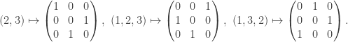
Now  acts on V by taking
  E.g. if n = 3, the representation is:
 be a cyclic group of order 3 and dim(V)=2. A representation of G is given by:
  Since this matrix is of order 3, the map is well-defined.
 Thus, dim(V) = #X. Now
 and the action of
![K[G]\times K[G]\to K[G]](https://s0.wp.com/latex.php?latex=K%5BG%5D%5Ctimes+K%5BG%5D%5Cto+K%5BG%5D&bg=ffffff&fg=333333&s=0&c=20201002) given by
given by  and extended linearly.
![K[G] \times V \to V](https://s0.wp.com/latex.php?latex=K%5BG%5D+%5Ctimes+V+%5Cto+V&bg=ffffff&fg=333333&s=0&c=20201002) to the basis
to the basis ![\{e_g : g\in G\} \subset K[G].](https://s0.wp.com/latex.php?latex=%5C%7Be_g+%3A+g%5Cin+G%5C%7D+%5Csubset+K%5BG%5D.&bg=ffffff&fg=333333&s=0&c=20201002) Since
Since  we get a representation of G on V.
 We’ll define a K[G]-module structure on V, by first decreeing that
 ![e_g\in K[G]](https://s0.wp.com/latex.php?latex=e_g%5Cin+K%5BG%5D&bg=ffffff&fg=333333&s=0&c=20201002) act on V via ρ(g), then extending linearly to the whole K[G]. Explicitly:
act on V via ρ(g), then extending linearly to the whole K[G]. Explicitly:![\begin{aligned}K[G] \times V\to V\end{aligned}](https://s0.wp.com/latex.php?latex=%5Cbegin%7Baligned%7DK%5BG%5D+%5Ctimes+V%5Cto+V%5Cend%7Baligned%7D&bg=ffffff&fg=333333&s=0&c=20201002) takes
takes 
 Now a typical element of K[G] is of the form:
 where
where 

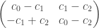 . This represents the action of
 ![c_0 + c_1 a + c_2 a^2 \in K[G]](https://s0.wp.com/latex.php?latex=c_0+%2B+c_1+a+%2B+c_2+a%5E2+%5Cin+K%5BG%5D&bg=ffffff&fg=333333&s=0&c=20201002) on V as a K[G]-module.
on V as a K[G]-module.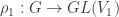 and
and  are both representations, then the direct sum
  gives:
 gives the matrix of g : V → V as
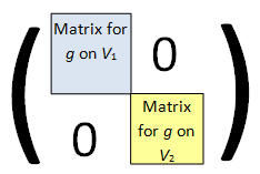
 the action of g on V results in
  Conversely, if W is a vector subspace of V which is invariant under all
 . Explicitly, if
  a basis of W, then
  gives a basis of the tensor product X.
 ; indeed, on elements
  this is easily seen to be true:
 the result follows. In terms of matrix representation, we get:
 is also a K[G]-module. To define the action of G on X, let’s imagine a K-linear map f : V → W written in the form of a huge lookup table (v, f(v)) such that each v occurs exactly once on the left. Now let G act on the entire table by replacing (v, f(v)) with the pair (g·v, g·f(v)). Unwinding the definition, we see that G acts on X via:


 on the left and the map
  on the right.
 .
. which is the image of
  and extended linearly.
 the restriction to
  is also a quotient map.
 is open. Hence
  for some open subset U of X. Then p(U) is open. We claim p(U) ∩ Z = V. Indeed,
  and
and  then
then  so
so  then since q is surjective, pick
  such that q(x)=y. Hence y lies in Z as well as p(U). ]
 is a subgroup of G and H/(H ∩ N) → (HN)/N is a bijective continuous homomorphism of topological groups.
 and is a dense subset:
 are both normal subgroups of G. Then we have an isomorphism of topological groups (G/N)/(H/N) → G/H.
 is continuous. But this map takes x to (x, 1/x) which is continuous since inverse is continuous on (R*, T). Hence, f is continuous.
 is continuous; the latter map takes (x, 1/x) to x, which is clearly continuous.
 is a homeomorphism. Indeed, the inverse is given by
  which is continuous.
 and
and 

 is trivial. This induces an action m’ : (G/N) × X → X which we claim is continuous. Since q : G × X → G/N × X is a quotient map, it suffices to show m’q is continuous. But m’q is precisely the original group action G × X → X, so we’re done.
 are ideals of R, then (R/I)/(J/I) is isomorphic to R/I as topological rings. Indeed, from classical ring theory, we have an isomorphism for the underlying ring structure. For the topology, we look at the underlying additive groups; by proposition 3, (R/I)/(J/I) and R/I are isomorphic topological groups. Hence, the two structures are isomorphic topological rings.
 of topological vector space V, (V/W)/(W’/W) and V/W’ are isomorphic vector spaces.
 This is a group under matrix multiplication since:
 and
and then Mt is its inverse and
 since the product and inverse maps are all given by polynomials in the matrix entries (inverse is particularly easy: it’s just the transpose).
 by:
by: ;
; just means
 where δij is the Kronecker delta function which returns 1 if i=j and 0 otherwise. In other words, M maps the standard basis to the orthonormal basis
  Hence a matrix in O(n) preserves the geometry of the Euclidean space by leaving distances and angles invariant.
 is closed since it’s defined by explicit polynomial equations in the matrix entries
  On the other hand, O(n) is bounded since each column vector of
 takes
takes  which is a continuous action. Let’s compute the isotropy group for x = en. This is the set of all
  we see that M must be of the form:
 , where


 and
and  .
. which drops the first coordinate is injective and continuous. The image is precisely the unit disc
  Since S+ is compact, the projection map is thus a homeomorphism onto D and so S+ is connected.
 , their union Sn-1 is also connected.
 for disjoint open subsets. If U contains a point x, it must contain the entire coset xH; otherwise,
  would be a partition of xH into disjoint open subsets, contradicting connectedness of xH.
 Since p is open,
  for disjoint open subsets p(U), p(V) of G/H. This must mean
  or
or  so U or V is empty.
 is open, so is p(U) by definition of quotient topology. ♦
 Then U = (1/2, 1] is open in I but p(U) is not open in S1.
  , then restricting to f : X → Z still gives an open map since if f(U) is open in Y, then f(U) ∩ Z = f(U) is open in Z.
 is open whether we use the product or box topology. To prove that, use the fact that for any map
  we have
 is open, then the resulting
  which takes
  is also open. Again, its proof requires
  if G/H is T1, then {e} is closed in G/H, hence H is closed in G.
 is closed in G/H × G/H. Now its complement is:
 is open since the continuous map
  gives us
 which is open since q is open. ♦
 and inverse map
  are continuous.
 is a collection of quotient maps which are open. Let
  be the projection map which takes
  .
. is open if and only if
  since q is surjective. Since each pi is open, so is q. And since q is surjective
  which must be open.
 is a continuous homomorphism of topological groups, this induces a continuous injective map
 where
where 
 is a closed normal subgroup N of G.
 is a homeomorphism. Thus, the connected components of G are the cosets gN, for various g. More generally, we’ll prove:
 which contains points from more than one connected component, so it is disconnected, i.e.
  for some non-empty disjoint open subsets U, U’ of Z.
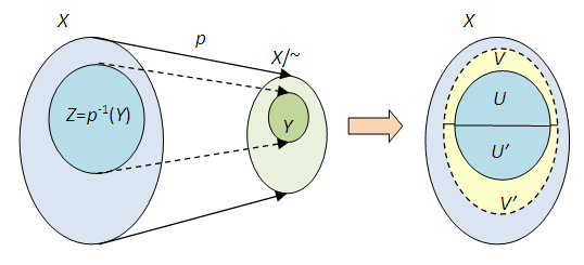
 as a disjoint union; since <x> is connected and
  we must have
  Thus U and U’ are both unions of connected components of X.
 ;
; : indeed, if it contains y, then pick
  such that p(x) = p(x’) = y. Then
  so they’re in U, U’ respectively. Since p(x) = p(x’), x and x’ must belong to the same connected component, which contradicts
 . The map
  which takes
  has kernel equal to Z. By theorem 5 above, this gives a bijective continuous homomorphism R/Z → S1. Since the image is Hausdorff, if we could prove R/Z is compact, then we’d have shown that R/Z and S1 are isomorphic topological groups. But then R/Z is the continuous image of the composition [0, 1] → R → R/Z. Case closed.
 . The same reasoning holds as before and one can show that R2/Z2 is isomorphic to S1 × S1.
 The determinant map GLn(R) → R* induces a bijective continuous homomorphism GLn(R)/SLn(R) → R*. Now we can’t use the same trick since the groups aren’t compact. Instead, we compose: R* → GLn(R) → GLn(R)/SLn(R) → R*, where the first map takes c to the diagonal matrix with entries (c, 1, …, 1). This gives the identity map on R*; since the first two maps are continuous, the last map is open.
 ]
]
 we would like the topology on Y to satisfy:
 , f is continuous if and only if
  is continuous.
 be a surjective map from a topological space X to set Y. The quotient topology on Y is defined as follows.
 is open if and only if
  is open in X.
 is continuous. For each open subset W of Z, the set
  is open in X. By definition of the quotient topology,
  is open in Y. ♦
 is closed in X.
 is surjective, does this give Z the quotient topology from X? [ Answer:
  , where
  Now:
Now:![f:[0, 1] \to S^1, \quad t \mapsto (\cos(2\pi t), \sin(2\pi t))](https://s0.wp.com/latex.php?latex=f%3A%5B0%2C+1%5D+%5Cto+S%5E1%2C+%5Cquad+t+%5Cmapsto+%28%5Ccos%282%5Cpi+t%29%2C+%5Csin%282%5Cpi+t%29%29&bg=ffffff&fg=333333&s=0&c=20201002)
 . By the universal property above, g is continuous since
 ![g\circ p = f :[0, 1]\to S^1](https://s0.wp.com/latex.php?latex=g%5Ccirc+p+%3D+f+%3A%5B0%2C+1%5D%5Cto+S%5E1&bg=ffffff&fg=333333&s=0&c=20201002) is continuous. Now, we invoke the lemma and conclude that g is a homeomorphism (together with the above exercise 5: since [0, 1] is compact, so is the quotient Y).
is continuous. Now, we invoke the lemma and conclude that g is a homeomorphism (together with the above exercise 5: since [0, 1] is compact, so is the quotient Y).

 gives Y’ the quotient topology from X’, then
  gives Y × Y’ the quotient topology from X × X’. But this is wrong, but a counterexample is fiendishly hard to find. For one, refer to Munkres, “Topology” (2nd ed.), section 22, page 145, exercise 6.
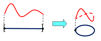
 be the unit disc on a plane. Collapse the outer circle comprising of points satisfying
  into a single point. The resulting topological space is homeomorphic to a 2-sphere:


 above.
 are all continuous too. Plus, they’re bijective and their inverses are given by
  respectively, which are all continuous. So the maps are homeomorphisms. ♦
 there’s a homeomorphism of G which maps x to y; indeed,

 which is a union of open subsets of G since right-multiplication is a homeomorphism. Same goes for BA. ♦
 which takes
  Clearly f is continuous, so
  is open. Now for any
  the ordered pair
  because if
  we would have
 for some open subsets
  and
and  such that
  By compactness of K, it can be covered by finitely many
 and
and 
 Thus
Thus  so indeed G–CK is open. ♦
 contains (x, e) so we have
  for some open subsets V, W of G containing x, e respectively.
 . Furthermore,
  since any element in the intersection corresponds to
  such that
  which is a contradiction. By proposition 2, (X–U)W is an open subset containing X–U, so any topological group is regular. ♦
 gives us
  Since cl(H) is a closed subset of G containing H,
  is a closed subset of G × G containing H × H. Thus
  which, together with
  , proves that cl(H) is a subgroup of G.
 is a homeomorphism and maps N to N. Thus it must map cl(N) to cl(N) also. ♦
 iff every open subset V containing x intersects H, which holds iff every open subset U containing e intersects
  And this holds iff
  Now recall that U is open iff
  is open. ♦
 Since left-multiplication by x is a homeomorphism of G, it must map the connected component of e to that of x. But x and e both have Y as their connected component, so xY = Y and thus
 where Un is the collection of products of n elements from U. It’s easy to see that V is an open subgroup of G. By the above proposition V is a clopen subset so V=G. It’s clear that the group <U> generated by U must contain V; thus <U>=G. ♦
 is a closed (resp. open) subgroup of G.
 which takes (a, b) to a+b√2. The homomorphism is clearly continuous if Z2 is given the discrete topology. However, the image of f is not closed.
 which takes (a, b) to a+b√2. This induces a group isomorphism from Z2 to im(f) which is continuous but not a homeomorphism.