
Character theory is one of the most beautiful topics in undergraduate mathematics; the objective is to study the structure of a finite group G by letting it act on vector spaces. Earlier, we had already seen some interesting results (e.g. proof of the Sylow theorems) by letting G act on finite sets. Since linear algebra has much more structure, one might expect an even deeper theory.
Some prerequisites for understanding this set of notes:
- basic group theory, up to group quotients and homomorphisms;
- linear algebra, including tensor product of vector spaces;
- elementary theory of (left) modules over non-commutative rings, including up to module quotients and homomorphisms.
[ We’ve yet to cover module theory and linear algebra; hopefully this will be rectified in the future. ]
At one point, one also needs to take the tensor product 

Throughout this document, G denotes a finite group and all linear algebra is performed over a field K. As time passes by, we’ll restrict ourselves to fields of characteristic 0, and then finally to the complex field C (or any of your favourite algebraically closed fields of characteristic 0). Also, all vector spaces over K are assumed to be of finite dimension.
Let’s begin.

G1. Group Representations and Examples
We define:
Definition. A representation of a group G is a group homomorphism
where V is a finite-dimensional vector space over field K.
If we fix a basis for V, then this is tantamount to giving a group homomorphism 
[ Note: throughout all notes on this site, matrix representation for a linear map is obtained via 
Just like the case of group actions, we can think of a group representation as providing a map:

which is conveniently denoted g·v instead. This satisfies 


Examples
- Let dim(V)=1 and G act trivially on it. Thus
takes every g to 1. We call this the trivial representation.
- Suppose
is the full symmetric group. Let dim(V)=1 and let G act on it via
where sgn(g) = +1 if g is an even permutation and -1 if it’s odd. This is called the alternating representation. Note that it’s only available for
and not for any old group.
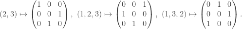
- Let
Now
acts on V by taking
E.g. if n = 3, the representation is:

- Let
be a cyclic group of order 3 and dim(V)=2. A representation of G is given by:
Since this matrix is of order 3, the map is well-defined.
Regular Representation
Example 3 above is clearly generalisable: if G acts on finite set X, then let V be a vector space with abstract basis 


In particular, any group G acts on itself by left multiplication, so this gives a representation of dimension #G. Explicitly, V is given an abstract basis 


This is called the regular representation of group G. Note that example 3 is not the regular representation since in the regular representation of S3, dim(V) = 3! = 6.
G2. The Group Algebra
We define:
Definition. Given field K and finite group G, the group algebra K[G] is a K-vector space with an abstract basis given by:
and multiplication
given by
and extended linearly.
Some concrete computations will make it much clearer. Suppose 
The following should now be clear.
Theorem. The group algebra K[G] is a ring which contains K as a subring. It is commutative if and only if G is abelian.
As a ring, we can talk about left modules over K[G]. These turn out to correspond precisely to representations of G.
Let’s do the easy direction first: suppose we’re given a left K[G]-module V. Then V is naturally a K-vector space and we obtain an action of G on V by restricting the left-module action ![K[G] \times V \to V](https://s0.wp.com/latex.php?latex=K%5BG%5D+%5Ctimes+V+%5Cto+V&bg=ffffff&fg=333333&s=0&c=20201002)
![\{e_g : g\in G\} \subset K[G].](https://s0.wp.com/latex.php?latex=%5C%7Be_g+%3A+g%5Cin+G%5C%7D+%5Csubset+K%5BG%5D.&bg=ffffff&fg=333333&s=0&c=20201002)

Conversely, suppose G acts on V via K-linear maps, i.e. every 
![e_g\in K[G]](https://s0.wp.com/latex.php?latex=e_g%5Cin+K%5BG%5D&bg=ffffff&fg=333333&s=0&c=20201002)
![\begin{aligned}K[G] \times V\to V\end{aligned}](https://s0.wp.com/latex.php?latex=%5Cbegin%7Baligned%7DK%5BG%5D+%5Ctimes+V%5Cto+V%5Cend%7Baligned%7D&bg=ffffff&fg=333333&s=0&c=20201002)

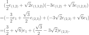
Concrete Example
Consider example 4 from section G1, where 


The corresponding matrix is then:

or 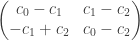
![c_0 + c_1 a + c_2 a^2 \in K[G]](https://s0.wp.com/latex.php?latex=c_0+%2B+c_1+a+%2B+c_2+a%5E2+%5Cin+K%5BG%5D&bg=ffffff&fg=333333&s=0&c=20201002)
G3. Creating New Representations
We’ll look at ways to create new representations of G from existing ones.
A. Direct Sum
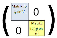
If R is a ring, then the direct sum of two R-modules is another one. In particular, this holds for R = K[G] as well. Specifically, if 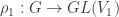


If we pick bases of V1 and V2, then the resulting basis of 
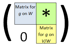
B. Submodules and Quotients
Generally, if M is a left R-module and 


If we pick a basis of W and extend it to V, then the matrix representation of
 C. Tensor Product
If V and W are K-vector spaces, we can take their tensor product over K: 


Given

Note that 


Since the set of all such elements spans 

D. Space of Linear Functions
Suppose V and W are K[G]-modules. The space of all K-linear maps 

Note that in the composition gfg-1, the left g acts on W while the right g-1 acts on V.
E. Dual Space.
A special case of the above is when W = K with the trivial representation. The resulting HomK(V, K) is known in linear algebra as the dual space V*. The above definition then gives us an action of G on V* via:

Let’s do some sanity check here. From linear algebra, there’s a canonical isomorphism:

If both V and W are K[G]-modules, then there appears to be two different ways to define a G-action on HomK(V, K). Fortunately, both ways are identical; this can be checked by letting 

- On the left, we get
.
- On the right, we get the composition
which is the image of
In a Nutshell
Given a finite group G and field K, we’ve defined the group algebra K[G] which is a ring containing K. This is done by using an abstract basis 
There’s a one-to-one correspondence between (1) K[G]-modules, and (2) linear representations of G on K-vector spaces.
The usual operations to construct new K[G]-modules are (A) direct sums, (B) submodules and quotients, (C) tensor products, (D) HomK(V, W) and (E) duals.
Everything presented so far is rather generic; in fact, one could even take K as any commutative ring and there’d be no effect on the theory thus far. In the next installation, we’ll explore the structure of K[G]-modules in greater detail.
