
First, suppose (X, d) is a metric space. If Y is a subset of X, then one can restrict the metric to 

The open subsets of Y are related to those of X as follows.
Proposition. A subset
is open if and only if
for some open
.
Proof.
First note that if 

- Suppose U is open in X and V = U ∩ Y. Each
is also in U, and so
for some ε>0. Hence
. So V is open in Y.
- Conversely, let V be open in Y. For each a in V, we have
for some ε>0 depending on a. Take the union U of all such
; then U is open in X since it’s a union of open balls in X. Also

Exercise
If U is an open ball in X, is U ∩ Y necessarily an open ball in Y?
[ Answer (highlight to read): no, consider X=R and Y=R-{0}. Then (-1, +1) is an open ball N(0, 1) in X but (-1, +1) ∩ Y is the disjoint union of (-1, 0) and (0, +1) which is not an open ball in Y. ]
This inspires us to extend the definition of subspaces to general topological spaces.
Definition. Let (X, T) be a topological space and Y be a subset of X. The subspace topology on Y is defined by:
i.e.
Equivalently, the class of closed subsets of Y is given by D = Y – (U∩Y) = (X–U) ∩ Y = C ∩ Y for some closed subset C of X.
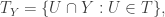
Examples
- A subspace of (X, d) with the discrete metric is still discrete.
- Pick the half-open interval
. Then
is open in Y but not open in R.
- Consider the subset
of the real line R. The singleton set {0} is an open subset of Y since {0} = N(0, 1/2). Furthermore, it is closed since the complement is a union of two open subsets.
- Consider the subset Z of R under the usual metric. Then the resulting subspace is the discrete space even though the induced metric d(m, n) = |m–n| is not exactly the discrete metric.
- Let
and Y be the set of points (x, y) satisfying
. Geometrically, Y is a circle. Here, we’ll think of it as a topological space with the subspace topology inherited from X. The space is denoted
. More generally, for each positive integer n, the space
is the subspace of
comprising of all points
satisfying
- Consider X = N under the right order topology.
- If Y = {1, 2, 3}, then the subspace topology gives { (empty set), {3}, {2, 3}, Y }.
- If Y is the set of even numbers, then the bijection
preserves the structure of topological spaces. We say that the two spaces are homeomorphic. We will say more about this in a later article.

 Since we’re often dealing with multiple spaces and subspaces, when describing open/closed subsets, it’s essential to qualify with “(XX) is open/closed in (YY)” instead of merely saying “(XX) is open”. E.g. in example 2 above, Y = [0, 1) is a subspace of R and the subset [0, 1/2) is open in Y but not in R.
The following diagram illustrates some open subsets of Y in example 3.
Exercises
- Consider the subspace Y = {1/n : n positive integer} of R, under the usual metric. Is this space discrete? What about
?
- Example 2 gives us the concept of clopen subsets, i.e. subsets of a topological space which are both open and closed. In any topological space X,
and X are always clopen. Are there any other clopen subsets of Q, where Q inherits the subspace topology from R?
Answers
- Y is discrete since each {1/n} = (1/n – ε, 1/n + ε) ∩ Y for some small ε>0. On the other hand Y* is not discrete since any open subset containing 0 must also contain some 1/n.
- Yes, Q has infinitely (in fact, uncountably) many clopen subsets. If r is irrational, then (-∞, r) ∩ Q and (r, ∞) ∩ Q form a disjoint union of Q by open subsets.
 Basic Properties of Subspaces

The following basic property is often taken for granted.
Theorem. If (X, T) is a topological space and
are subsets, then we can form the subspace topology on Z in two ways:
- by taking the subspace topology
from
; and
- by taking successive subspaces
which is a topology on Y, then
.
The two topologies are identical.
The proof is straightforward: in the first case, the class of all open subsets of Z is given by U ∩ Z for open subsets U of X; in the second case, the class is given by (U ∩ Y) ∩ Z = U ∩ Z for open subsets U of X. They’re identical. ♦
The following properties are also surprisingly useful in practice.
Theorem. Let Y be a subspace of (X, T). If Y is open in X, then any open subset of Y is an open subset of X. If Y is closed in X, then any closed subset of Y is a closed subset of X.
Proof.
For the first statement, an open subset of Y is of the form V = U ∩ Y for some open subset U of X. Since U and Y are both open in X, so is V = U ∩ Y. The same proof holds for the second statement by replacing ‘open’ with ‘closed’. ♦
Furthermore, for bases and subbases, we have:
Theorem. Let
be a topological space with subspace
.
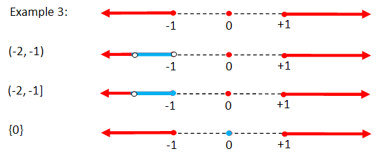
- If B is a basis for T, then
is a basis for Y.
- If S is a subbasis for T, then
is a subbasis for Y.

Proof.
For the first statement, we first verify that 
- Any two elements of
for some basic open subsets
. Since B is a basis,
for some
. This gives
which is a union of elements in

Finally, we need to show 
- Every element
(for some element U in B) is open in Y by definition. So
.
- Conversely, any element of
for some open subset U of X. Since B is a basis for (X, T),
for some
. So
which is a union of elements in
This concludes the proof for the first statement.
For the second, suppose the intersections of finitely many elements of S form basis B. It suffices to show that the intersections of finitely many elements of 
- In one direction, note that
.
- Conversely, any element of
. So
for finitely many
. But this gives
for finitely many
.
And the proof is complete. ♦
Summary.
- Any subset of a topological space X inherits a topology from it. The inheritance is consistent across inclusion chains of topological spaces.
- With spaces and subspaces, one should be more careful when talking about “open sets”, i.e. mention what it’s open in.
- If Y is open (resp. closed) in X and Z is open (resp. closed) in Y, then Z is open (resp. closed) in X.
- If Y is a subspace of X, then a basis (resp. subbasis) of X restrict to give a basis (resp. subbasis) of Y.
 is contained in some open ball
  for some ε>0 which depends on x; hence U is the union of all these N(x, ε).
 such that every open subset U of X is a union
  a basic open set.
 is some collection of subsets of X. Is it always the basis of some topology?
 , so no problem there; for X, we need to specify that
  .
. (where each
  ) is also of the form
  which lies in T.
 and
and  , with each
  . Since intersection is distributive over union, we get:
 for all
  . On the other hand, this condition is obviously necessary since if
  . Thus we have proven:
 is a union of elements from B.
 corresponds to solutions of simultaneous linear congruences
  ,
,  . From elementary number theory, this intersection is either empty or V(e, f) for some integers e, f (where e = lcm(a, c)). Since V(1, 0) = Z, {V(a, b)} forms a basis for some topology T on Z.
 is a collection of topologies on X, one easily checks that so is
  where a subset of X is open in T if and only if it’s open in all Ti. In short, an intersection of topologies is still a topology; so given any subset
  , one can consider the collection of all topologies containing S (this is a non-empty collection since it includes the discrete topology) and take their intersection.
 ;
; .
.
 , we have
  too, since T is the smallest topology containing S.
 , for some
  , then since
  , we have
  as well. Thus,
  . ♦
. ♦
 be the power set of X (i.e. set of all subsets of X). A topology on X is a subset
  satisfying:
 ;
; , then
  ;
; is a collection of elements of T, then
  .
. are open, then so is
  . In other words, a topology is closed under an intersection of finitely many terms, but not infinitely many terms in general (see the example of R later, where the intersection of all
  is {0}, which is not open).
 are closed subsets of X;
 are closed subsets of X, then so
  is closed;
 is a collection of closed subsets of X, then
  is closed.
 are both topologies on X. If
  , then we say
  is a finer topology than
  and conversely
 , which is the coarsest topology possible for X.
 . The standard topology on X was already defined
  for m=1, 2, 3, … . Note that
  and
and  ; the fact that the order topology is closed under arbitrary union follows from that every subset of N has a minimum.
 , where ∞ is just a dummy symbol here, then we can define a topology on N* by decreeing that the only non-empty open subsets are
  Thus, any open subset containing ∞ contains all sufficiently large natural numbers.
 such that:
 .
. and
and  . [ See diagram below. ]
 where
where  is the highest power of p dividing m; in the case m=0, since all powers of p divide m we have
  . Then
  is a metric, called the p-adic metric on Z. This was briefly alluded to in a

 for some ε>0. Then the collection of open sets form a topology.
 are open (in the sense of metric space). If
  , then x lies in both U1 and U2. Thus, we can find
  such that:
 and
and  .
. .
. be open and
  . If x lies in U, then it must lie in some Ui. Thus, for some ε>0,
  . ♦
. ♦ induces the topology on Rn defined earlier;
 ;
; ;
; , i.e. it is open in the metric space (X, d). Then for any x in U,
  for some ε>0. By the first condition,
  for some δ>0. Hence it follows that U is open in the metric space (X, d’) too.
 is open in T, it is also open in T’. Hence
  for some δ>0. ♦
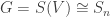 then acts on E. Each graph corresponds to a colouring of E by Y = {black, white} and two graphs are isomorphic if and only if they’re isotopic under G – i.e. belong to the same orbit under G. Our objective is to compute the number of unique colourings by applying Polya enumeration theorem.
 acts on X by permuting the edges around.
 .
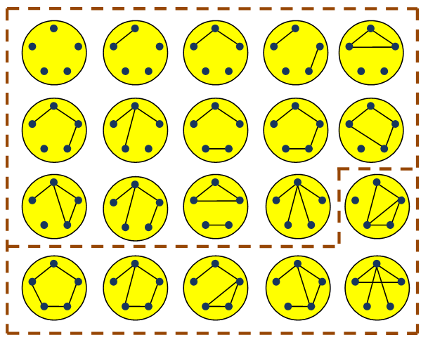
. , the number of isomorphic classes of simple graphs with 5 vertices and i edges.
 . Burnside’s lemma gives:
 for each g.
 , this is just
 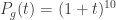 .
. . For the remaining 4 singleton orbits, we get a factor of
  , so the summand is
  .
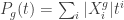
. while the singleton set contributes (1+t), hence the summand is
  .
.

 . Thus, there are 1 graph with 1 edge, 2 graphs with 2 edges, 4 graphs with 3 edges, … up to isomorphism.
 is the number of cycles (or orbits) in g of length c.
 ;
; ;
; , so we have
  .
.
 be the set of colourings with weight i, then our objective is to compute
 , for each g in G.
 where
where  is the number of colours of weight w. Hence:
 , this gives:
  . Summing up:
 . Then the number of colourings with a specified weight is given by the generating function:
 .
. as we saw above.


 ;
;
 denotes the number of colours of weight (v, w). Then Polya’s enumeration theorem can be further generalised: the number of colourings with a specified vectorial weight (v, w) is given by the coefficient of
  in:
in:


![\begin{aligned} P(t, u)= &\frac 1 {24}[(1+t+u)^{12} + 6(1+t^4+u^4)^3 + 3(1+t^2+u^2)^6\\&+6(1+t+u)^2 (1+t^2+u^2)^5 + 8(1+t^3+u^3)^4].\end{aligned}](https://s0.wp.com/latex.php?latex=%5Cbegin%7Baligned%7D+P%28t%2C+u%29%3D+%26%5Cfrac+1+%7B24%7D%5B%281%2Bt%2Bu%29%5E%7B12%7D+%2B+6%281%2Bt%5E4%2Bu%5E4%29%5E3+%2B+3%281%2Bt%5E2%2Bu%5E2%29%5E6%5C%5C%26%2B6%281%2Bt%2Bu%29%5E2+%281%2Bt%5E2%2Bu%5E2%29%5E5+%2B+8%281%2Bt%5E3%2Bu%5E3%29%5E4%5D.%5Cend%7Baligned%7D&bg=ffffff&fg=333333&s=0&c=20201002)
 where i and j are both even, compute the sum
 . ♦
. ♦ . In the

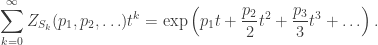
 is given by the generating function:
 is the i-th power symmetric function. The question is: how many colourings are of weight
  and 0 otherwise. Now if we multiply this by an auxiliary
  and sum over all k=|X|, we get the resulting power series:
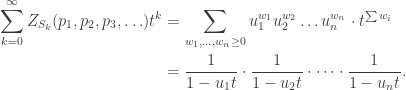

 , let
, let 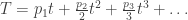 . We need to compute the expansion of exp(T) until T5 and find the coefficient of t5.
 ;
; ;
; ;
; ;
; .
.
 , there are:
 colourings since each vertex can take n colours independently. Letting X denote the set of these colourings, the group S3 acts on X by permuting the vertices. Our objective is now to compute
  , the number of orbits under this group action. To that end, the following result is phenomenally useful.
 ,
, is the set of all elements of X fixed by g.
 . We’ll compute |S| in two ways.
  , the RHS.
 , where
  is the isotropy group of x and
  , where Gx is the orbit of x. Hence,
 ,
, for each element
  :
: ;
; ;
; .
. ♦
♦ , which is the set of all functions X→Y. The action of G on X extends to an action on S as follows:
 and
and  is a colouring, then the action is given by the composition
 .
. . ]
. ] . But
. But  is not hard to compute: if we express the action of g on X as a permutation, and c(g) denotes its number of cycles (or orbits), then
  since the points in each cycle must share the same colour. This gives:
 , where n = |Y|.
 ,
, as above. Let’s consider more examples.
 .
. which is precisely the number of ways to colour the four vertices of a square with n colours, up to rotational/reflection symmetry. ♦
 , consider the number of orbits c((g, h)). This only depends on the conjugancy classes of g and h. For example:
 . ♦
. ♦
 is the number of elements
  with exactly c orbits.
 ,
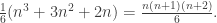
, is the number of occurrences of colour i. Elementary combinatorics then tell us the number of solutions is:
 .
. in the polynomial:
 .
.![\left[\begin{matrix}k\\c\end{matrix}\right]](https://s0.wp.com/latex.php?latex=%5Cleft%5B%5Cbegin%7Bmatrix%7Dk%5C%5Cc%5Cend%7Bmatrix%7D%5Cright%5D&bg=ffffff&fg=333333&s=0&c=20201002) and is called a Stirling number of the first type.
and is called a Stirling number of the first type.
![\left[\begin{matrix}n+1\\k\end{matrix}\right] = n\left[\begin{matrix}n\\k\end{matrix}\right] + \left[\begin{matrix}n\\k-1\end{matrix}\right]](https://s0.wp.com/latex.php?latex=%5Cleft%5B%5Cbegin%7Bmatrix%7Dn%2B1%5C%5Ck%5Cend%7Bmatrix%7D%5Cright%5D+%3D+n%5Cleft%5B%5Cbegin%7Bmatrix%7Dn%5C%5Ck%5Cend%7Bmatrix%7D%5Cright%5D+%2B+%5Cleft%5B%5Cbegin%7Bmatrix%7Dn%5C%5Ck-1%5Cend%7Bmatrix%7D%5Cright%5D&bg=ffffff&fg=333333&s=0&c=20201002)
![\left[\begin{matrix}n\\n-2\end{matrix}\right] = \frac 1 4(3n-1){n\choose 3}](https://s0.wp.com/latex.php?latex=%5Cleft%5B%5Cbegin%7Bmatrix%7Dn%5C%5Cn-2%5Cend%7Bmatrix%7D%5Cright%5D+%3D+%5Cfrac+1+4%283n-1%29%7Bn%5Cchoose+3%7D&bg=ffffff&fg=333333&s=0&c=20201002)
![\left[\begin{matrix}n\\2\end{matrix}\right] = (n-1)! (1 + \frac 1 2 + \frac 1 3 + \dots + \frac 1 {n-1})](https://s0.wp.com/latex.php?latex=%5Cleft%5B%5Cbegin%7Bmatrix%7Dn%5C%5C2%5Cend%7Bmatrix%7D%5Cright%5D+%3D+%28n-1%29%21+%281+%2B+%5Cfrac+1+2+%2B+%5Cfrac+1+3+%2B+%5Cdots+%2B+%5Cfrac+1+%7Bn-1%7D%29&bg=ffffff&fg=333333&s=0&c=20201002) .
. , the following are equivalent.
 , such that 0 < |xn–x| < 1/n for each n. Then (xn)→x must be in L.
 . Since a is not in D it’s not a point of accumulation of D. By definition, this means that there exists ε>0 such that the set of x satisfying 0 < |x–a| < ε does not intersect D. Together with the fact that a is not in D, we see that
  , so Dc is open.
 , an open subset of R, there must be an open ball
  . On the other hand, since (xn)→L, some
  is a closed subset if D-U is an open subset of D.
 , x > M-ε and x < M. This shows that M is a point of accumulation of D, and by the above proposition, it must lie in D, which contradicts our assumption. Thus M is a maximum of D. The case for minimum is similar.
![D = [1, 2]\cup \{3\}](https://s0.wp.com/latex.php?latex=D+%3D+%5B1%2C+2%5D%5Ccup+%5C%7B3%5C%7D&bg=ffffff&fg=333333&s=0&c=20201002) . It is closed in R since the complement is
. It is closed in R since the complement is  which is a union of open intervals. Clearly D is bounded. Being both closed and bounded, it has a minimum and a maximum (in this case, 1 and 3 respectively).
 . It is not closed because its complement is
  and the point 2 has no open neighbourhood of R which is wholly contained in E. Or, look at it another way, if it were closed, then since it’s obviously bounded it would contain a maximum and a minimum, but 2 is the supremum of D which is not contained in D itself.
 . The complement is
  which is a union of open intervals and is hence open. But it’s not upper-bounded so it doesn’t have a maximum.
 is closed in D.
 .
.
 is uniformly continuous (on D) if:
 and
and  ,
, is Cauchy but the resulting
  is not a Cauchy sequence. Hence, this tells us f(x) is not uniformly continuous, as we had verified earlier directly in example 2 above.
 is a sequence of uniformly continuous functions on D, which converges uniformly to
  . Fix n. Since
  is uniformly continuous, there exists δ>0 such that whenever
  satisfies |x–y|<δ, we also have
  . Hence:
 .
. , where n = 1, 2, 3, … ,
 converges to some real value. We’ll denote this value by f(x), thus defining a function f : D → R. We then say that the sequence of functions fn(x) converges to f(x) pointwise.
![f_n : [0,1]\to\mathbf{R}, \quad f_n(x) = x^n.](https://s0.wp.com/latex.php?latex=f_n+%3A+%5B0%2C1%5D%5Cto%5Cmathbf%7BR%7D%2C+%5Cquad+f_n%28x%29+%3D+x%5En.&bg=ffffff&fg=333333&s=0&c=20201002)


 and
and  ,
, ♦
♦
 which is either a non-negative real number or +∞. It’s not hard to show that
  ,
,  and
and  .
. uniformly if:
 on D=[0,1]. Since the functions converge to a discontinuous function, the above theorem tells us the convergence is not uniform, but let’s verify this directly. Indeed, the function
  takes xn on [0,1) and 0 at x=1. Thus,
  for all n, which shows that the convergence is not uniform.
 for each n, so
  . As expected, since each fn(x) is continuous, so is the resulting converged function f(x).
 for each n. In other words, one can have pointwise convergence of a sequence of continuous functions to a continuous function, even if the convergence is not uniform.
 on (1, ∞). We know
  , so that
  pointwise. Suppose we wish to show that ζ(x) is continuous at x=a>1.
 which is a convergent series since b>1.
 , which shows that gn converges uniformly to g.
 and
and  are sequences of functions which converge uniformly to
  respectively. What about the sum
  , product
  and reciprocal
  ?
? uniformly. To see why, write:
 ,
,  and
and  for large n. Thus, we also have
  for large n.
 for large n. It then follows that we can write
  for some positive bound B and
  . Hence, it also follows that
  converges uniformly.
 and
and  uniformly. However,
  .
. uniformly, assuming that g(x) and gn(x) are never 0. Taking the difference gives:
 for all n. This means
  for all n, and
  , i.e.
  for all n>N and
  when
when  .
. for all n and it follows that
  is zero? Consider the example of
 ![g_n: (0, 1]\to\mathbf{R}, g_n(x)=(1+\frac 1 n)x](https://s0.wp.com/latex.php?latex=g_n%3A+%280%2C+1%5D%5Cto%5Cmathbf%7BR%7D%2C+g_n%28x%29%3D%281%2B%5Cfrac+1+n%29x&bg=ffffff&fg=333333&s=0&c=20201002)
 . Then
  converges to g(x)=x uniformly since
  . On the other hand,
 and
and  uniformly, where each
  . Then:
 uniformly as well;
 , then
  for all n, then
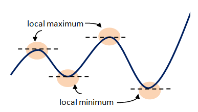
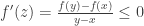
 . Now when x>a, we have f(x)≤f(a), so
  and so the limit ≤ 0. On the other hand, when x<a, the inequality f(x)≤f(a) also gives
  so the limit ≥ 0. These two inequalities force the limit to be 0. ♦
 is closed if its complement Rn-C is an open subset of Rn. We’ll have more to say about closed subsets in a later article.
 . Now to form a triangle, we need L/2 ≤ a ≤ L which gives a function f : [L/2, L] → R. Since [L/2, L] is closed and bounded, the image of f attains a maximum and a minimum.
 gives us x=L or (2/3)L. Clearly, the latter is the correct answer. So the optimum dimensions are (2L/3, 2L/3, 2L/3), an equilateral triangle.
 ;
; ;
; .
. . Since b varies, we differentiate this with respect to b and set it to zero, which gives b = L-(a/2), i.e. the sides are a, L-(a/2) and L-(a/2) so we get an isosceles triangle, which reduces this to the previous problem.
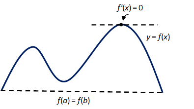
 .
.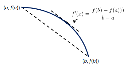
 , for some constant c such that g(a) = g(b). Clearly,
  . Rolle’s theorem says there exists x in (a, b) such that g’(x) = 0, whence we have
  . ♦
. ♦ , which is a contradiction. ♦
 . Let’s check the behaviour of f(x) as x increases. The above results suggest that the derivative is helpful: indeed, writing
  gives:
 which contradicts the second point. Likewise, if x < e satisfies f(x) ≥ f(e), then this contradicts the first point.
 .
. ,
, for all x in (a, b), x ≠ c,
 ,
, .
.
 to converge. E.g. take our earlier example of
  and g(x) = x, defined on x≠0. Then the first two conditions are satisfied, but now
 by squeeze theorem. In summary, even if f’(x)/g’(x) fails to converge as x→c, it’s still possible for f(x)/g(x) to converge.
 if
if  . [ Note that the converse isn’t true, as the above warning tells us. ]


 ,
,  . The resulting function is then written as
  .
.

 when x≠a. Hence, as x→a, the expression tends to
  . Conclusion: the derivative exists at every point a on the real line and
  .
. .
. . Conclusion: the derivative exists for every non-zero a.
 , so:
, so:


 ,
,
 ,
, .
. ;
; ;
; ;
; .
.
 for n≥0. By applying the division rule, we see that in fact this equation holds for all integers n.
 . We wish to compute
  and
and  . Since f(x) = v(u(x)), the chain rule gives us

 . Substituting x=1 then gives us the combinatorial equality:

 on the LHS and
  on the RHS by using the chain rule with u(x) = 1-x. But there’s no guarantee that the addition rule holds for infinitely many terms, although in this case it does work. The underlying theory will be covered in greater detail in a later article.

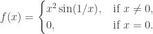 When a≠0, the derivative
  , which does not converge as a→0. When a=0, the derivative is
  by squeezing the function between |x| and -|x|.
 At the points x=a≠0, it’s easy to see the n-th derivative is of the form
  for some polynomial p(x) and positive integer m. To check its behaviour as x→0, let y=1/x; then
  which approaches zero since exponential increases much faster than any polynomial function. With this, one proves via induction that the n-th derivative at 0 is always 0, so the Taylor series is 0.
 where
where  . To that end, we need the Euclidean distance function on Rn. If x = (x1, x2, …, xn) is in Rn, we define:
 is said to be continuous at a if:
 is said to be a point of accumulation, if for any ε>0, there exists
  such that
 .
.
 is continuous.
 and
and  is continuous at a and
  is continuous at b=f(a), then
  is continuous at a.
 which projects to i-th component is continuous at every point.
 is continuous for each i.
 are continuous, as is the reciprocal
  .
. .
. for each i=1,2,…,m. Hence, when x is close to a in D, we have |f(x)-f(a)| < ε as well.
 . When |x–a|<|a|/2, we have |x|>|a|/2. Hence, for any ε>0, whenever |x–a|<min(|a|/2, ε|a|2/2) we get
  .
. and
and  are continuous at a and a’ respectively, where
  . Then
  given by
  is continuous at (a, a’).
 is continuous if it’s continuous at every point in the domain. From definition, it’s clear that continuity at a specific point is determined by what happens close to that point. To that end, let’s define open sets.
 is the set of points:
 . ]
. ] is said to be an open subset of D if for each
  for some ε>0.
 . Indeed, any y in N(x, δ) satisfies
![D = [0, 1]\cup\{2\}](https://s0.wp.com/latex.php?latex=D+%3D+%5B0%2C+1%5D%5Ccup%5C%7B2%5C%7D&bg=ffffff&fg=333333&s=0&c=20201002) . The subset U = [0, 1] is now an open subset of D. This may confuse the reader at first glance, but note that even if we pick the endpoint 1 (in U), we can pick the open ball N(1, 1/2) in D. By definition, this is the set
. The subset U = [0, 1] is now an open subset of D. This may confuse the reader at first glance, but note that even if we pick the endpoint 1 (in U), we can pick the open ball N(1, 1/2) in D. By definition, this is the set  , so it’s (1/2, 1] which is wholly contained in U. Likewise, the singleton subset V = {2} is also a subset of D, since the open ball N(2, 1/2) = {2} is wholly contained in U.

 while in the other two,
  . The dotted boundary lines indicate that the boundaries are not included in U.
 ,
,  is an open subset of D.
 . Since f(a) is in U which is open, there exists an ε>0 such that N(f(a), ε) is a subset of U. And since f is continuous at a, there exists a δ>0 such that whenever |x–
 is open for any open subset
  is open, so is
 .
.