Mathematics and Such

Topology: Separation Axioms

Posted on March 15, 2013 by limsup

Motivation

The separation axioms attempt to answer the following.

Question. Given a topological space X, how far is it from being metrisable?

We had a hint earlier: all metric spaces are Hausdorff, i.e. distinct points can be separated by two disjoint open subsets. But that’s only part of the story. Metric spaces, in fact, satisfy more.

Theorem 1. If (X, d) is a metric space and $C, D\subset X$ are disjoint non-empty closed subsets, then we can find open subsets U, V of X such that:

$U\supseteq C,\ V\supseteq D,\ U\cap V=\emptyset.$

To prove this, let’s have a little lemma. [ Note: this will be important later; it pays to take note of it now. ]

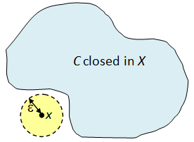
Lemma. Let C be a closed subset of a metric space (X, d) and $x\in X-C.$ Then the distance from x to C:

$d(x, C) := \inf\{ d(x,y) : y\in C\}$

is positive.

Proof of Lemma.

Since $x\in X-C$ and X–C is open, there is an ε>0 such that $N(x,\epsilon) \subseteq X-C.$ It follows that any y in C satisfies d(x, y) ≥ ε so $d(x,C)\ge \epsilon.$ ♦

Now we’re ready to prove the theorem.

Proof of Theorem.

For each $x\in C$ , we have d(x, D) > 0. Take the union of all $N(x, \frac 1 2 d(x,D))$ over $x\in C$ and call this set U; this is an open set containing C. Likewise, take the union of all $N(y, \frac 1 2 d(y,C))$ over all $y\in D$ and call this set V, which is an open set containing D.

We claim U and V are disjoint. If not, z lies in both $N(x, \frac 1 2 d(x,D))$ and $N(y, \frac 1 2 d(y,C))$ for some $x\in C, y\in D.$ This gives:

$d(x,z) < \frac 1 2 d(x,D),\ d(y,z) < \frac 1 2 d(y,C) \implies d(x,y)< \frac 1 2(d(x,D) + d(y,C)).$

But by definition d(x, y) ≥ d(x, D) and d(y, x) ≥ d(y, C), which is a contradiction. ♦

Separation Axioms

Let X be any topological space now. The following labels are given to X if it satisfies the corresponding condition:

Definition.

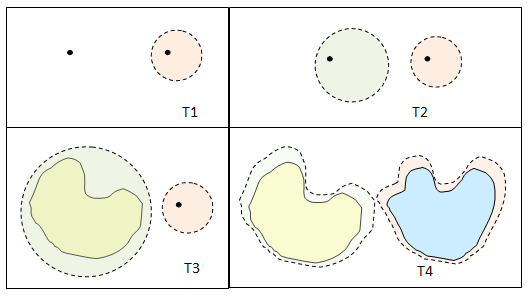
T1 : for any distinct points $x,y\in X,$ we can find an open subset U of X containing x but not y.

T2 : for any distinct points $x,y\in X,$ we can find open subsets U, V of X, such that $x\in U, y\in V, U\cap V=\emptyset.$

T3 : T1 and regular (X is regular if, for any point $x\in X$ and closed subset C of X not containing x, we can find open subsets U, V of X, such that $x\in U, C\subseteq V, U\cap V=\emptyset$ ).

T4 : T1 and normal (X is normal if, for any disjoint closed subsets $C, D\subseteq X,$ we can find open subsets U, V of X such that $C\subseteq U, D\subseteq V, U\cap V=\emptyset$ ).

Note that T2 is just the Hausdorff condition. Theorem 1 thus says: a metric space satisfies all the separation axioms.

Let’s examine these axioms one at a time.

Proposition 2 (T1). The space X is T1 if and only if all singleton sets {x} are closed.

Proof.

(→) If X is T1, let C = {x}. For any y outside x, the T1 axiom tells us there’s an open subset V containing y but not x, i.e. $y\in V\subseteq X-C.$ Hence X–C is open.

(←) If x, y are distinct points in X, then X-{y} is open and it contains x but not y. ♦

Note.

This proposition explains why, for T3 and T4, we have to specify the condition of T1 in addition to regularity / normality. This ensures that each {x} is closed and so T4 → T3 → T2 → T1, in increasing order of generality.

Furthermore, none of the implications is reversible. E.g. the topology (X, T) with X = {1, 2} and T = {{}, {1}, {1, 2}} satisfies T1 but not T2. For other examples, the reader may search the “spacebook” which is based on the famous book “Counterexamples in Topology“.

Proposition 3 (T3). A locally compact Hausdorff space is T3.

Proof.

Note that a space X is regular if and only if for any open subset U of X and $x\in U,$ there’s an open subset V of X satisfying $x\in V\subseteq \text{cl}(V)\subseteq U.$

Now suppose X is locally compact and Hausdorff. Let U be an open subset of X containing x. By theorem 1 here, x is contained in an open subset V of X such that cl(V) is compact and contained in U. ♦

The converse is not true: there’re T3 spaces which are not locally compact. Also, there’re locally compact spaces which are not T4.

Proposition 4 (T4). A compact Hausdorff space is T4.

Proof

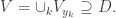
Suppose X is compact; then it’s locally compact so it’s T3. Let C, D be disjoint closed subsets of X. For each $y\in D,$ since X is T3, we can pick open subsets:

$U_y\supseteq C,\ V_y\ni y,\$ such that $U_y\cap V_y = \emptyset.$

Now the collection of {V_y} covers D. Since D is a closed subset of compact X, it’s compact as well, so there’s a finite subcover $\{V_{y_k}\}\subseteq \{V_y\}.$ Let:

$U := \cap_{k=1}^n U_{y_k},\ V := \cup_{k=1}^n V_{y_k}.$

Since U_y and V_y are disjoint for each y, so are U and V. We get: $U = \cap_k U_{y_k} \supseteq C$ and $V = \cup_k V_{y_k} \supseteq D.$ ♦

Clearly, not every T4 space is compact since there’re metric spaces which are not compact.

Combined Properties

The separation axioms satisfy the following properties. We skip the case of T2 since it had been done earlier.

Theorem 3. If Y is a subspace of X, and X satisfies T1 (resp. T2, T3), then so does Y.

Proof.

(T1). If $y\in Y,$ then {y} is closed in X since X satisfies T1. So {y} ∩ Y = {y} is closed in Y.

(T3). Let D be a closed subset of Y and $x\in Y-D.$ Denote $C = \text{cl}_X(D)$ which is closed in X. Since

$D = \text{cl}_Y(D) = \text{cl}_X(D) \cap Y = C\cap Y$

we see that C doesn’t contain x. Since X is regular, we can enclose x, C in disjoint open subsets U, V of X. Then $D = C\cap Y\subseteq V\cap Y$ and $x\in U\cap Y$ where U ∩ Y and V ∩ Y are disjoint open subsets of Y. ♦

Exercise.

Prove that if Y is a closed subset of X and X satisfies T4, then so does Y. [ A subspace of a T4 space is not necessarily T4, but counter-examples are hard to find. ]

Theorem 4. If $\{X_i\}$ is a collection of topological spaces which satisfy T1 (resp. T2, T3), then so is their product $X:= \prod_i X_i.$

Proof.

(T1). Let $(x_i) \in X.$ If each X_i is T1, then the singleton set $\{x_i\}\subset X_i$ is closed. Since a product of closed subsets is closed, it follows that $\{(x_i)\} \subset X$ is also closed. Hence, X is T1.

(T3) Let $\mathbf{x} := (x_i) \in X$ and $C\subseteq X$ be a closed subset of X not containing x. Then X–C is an open subset of X containing x so it contains a basic open subset:

$\mathbf{x} \in \prod_i U_i \subseteq X_i,$ for some open $U_i\subseteq X_i,$

where equality holds for $i\ne i_1,\ldots, i_n.$ Then $x_i\in U_i$ for each i. For each $i=i_1, \ldots, i_n,$ since X_i is regular, there’s an open subset V_i of X_i such that $x_i\in V_i\subseteq \text{cl}(U_i)\subseteq U_i.$ For the remaining $i\ne i_1, \ldots, i_n$ we set V_i := X_i.

Now $\prod_i V_i$ is open and:

$\mathbf{x}=(x_i) \in \prod_i V_i \subseteq \text{cl}(\prod_i V_i) = \prod_i \text{cl}(V_i) \subseteq \prod_i U_i.$ ♦

Note

Unfortunately, a product of T4 spaces is not necessarily T4.

Urysohn’s Lemma

Urysohn’s Lemma. Suppose X is normal. Then for any disjoint non-empty closed subsets C, D of X, there is a continuous map $f:X\to [0,1]$ such that f(C)={0} and f(D)={1}.

[ In particular, this holds for T4 spaces. ]

Note.

If X is connected, then f must be surjective since f(X) is a connected subset of [0, 1] containing 0 and 1. So we can label points of X continuously from 0 to 1 without gaps!

Proof.

[ All closed/open subsets are assumed with reference to X. ]

Note that normality is equivalent to: for any closed C and open U containing it, there’s an open V and closed D such that $C\subseteq V\subseteq D\subseteq U.$

Armed with this, first define $C_0 := C$ and $V_1 := X-D \supseteq C_0.$ For the first step, let $V_{1/2}$ be open and $C_{1/2}$ be closed such that $C_0 \subseteq V_{1/2} \subseteq C_{1/2}\subseteq V_1.$

Now proceed inductively, suppose we have a sequence of sets (each “C” is closed and “V” is open):

$C_0 \subseteq V_{1/2^k} \subseteq C_{1/2^k} \subseteq \ldots \subseteq V_{r/2^k} \subseteq C_{r/2^k}\subseteq V_{(r+1)/2^k} \subseteq \ldots \subseteq V_1.$

For each 0 ≤ r/2^k< 1, given the inclusion $C_{r/2^k} \subseteq V_{(r+1)/2^k},$ find open $V_{(2r+1)/2^{k+1}}$ and closed $C_{(2r+1)/2^{k+1}}$ such that:

$C_{r/2^k} \subseteq V_{(2r+1)/2^{k+1}}\subseteq C_{(2r+1)/2^{k+1}} \subseteq V_{(r+1)/2^k}.$

This creates a corresponding chain for r/2^k+1. In this way, we create a series of $V_r$ and $C_r$ for each dyadic rational number (i.e. of the form r/2^k) between 0 and 1.

Now define the function:

$f:X \to [0,1], \quad f(x) = \inf\{t : x\in V_t \text{ or } t=1\}.$

Clearly f(C) = {0} and f(D) = {1}. It remains to show f is continuous.

Let $U_b=f^{-1}([0, b))$ for b>0. Now the inf of a set is less than b iff some element of the set is less than b, so $U_b=\cup_{t<b} V_t$ is open.

Let $C=f^{-1}([0, b])$ for some b≥0. Now if t>b and $x\in C,$ then f(x)<t so $x\in V_t \subseteq C_t.$ This means $C\subseteq \cap_{t>b} C_t.$ Conversely, if f(x) > b, then there’re dyadic t, u such that f(x) > t > u > b. Then $x\not\in V_t$ and so $x\not \in C_u \implies x\not\in \cap_{t>b} C_t.$ Hence $C = \cap_{t>b} C_t$ is closed and $f^{-1}((b, 1])$ is open.

Since [0, b) and (b, 1] form a subbasis for [0, 1], we’re done. ♦

Urysohn’s Metrisation Theorem

The following result shows a sufficient condition for metrisability.

Definition. A topological space X is second-countable if it has a basis B with countably many elements.

For example, even though set-theoretically R is uncountable, its topology is second-countable since it has a basis comprising of open intervals (a, b) for rational a<b.

Urysohn’s Metrisation Theorem. If X is a T3 space which is second-countable, then it’s metrisable.

The proof follows a couple of steps.

Step 1 : T3 + second-countable implies T4.

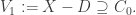
Let $C, D\subseteq X$ be disjoint closed subsets. For each $x\in C$ , since X is T3, we can find an open subset U_x containing x such that its closure is disjoint from D. Since X has a countable basis and $C \supseteq \cup_x U_x,$ we can find a countable subcover

$C\supseteq \cup_{n=1}^\infty U_{x_n},$ with each $\text{cl}(U_{x_n})\cap D = \emptyset.$

Similarly, we’ll cover D via $D\supseteq \cup_{n=1}^\infty V_{y_n}$ with each $\text{cl}(V_{y_n})\cap C =\emptyset.$ Now define:

$U_n' = U_{x_n} -(\text{cl}(V_{y_1}) \cup \ldots \cup \text{cl}(V_{y_n}))$ and $V_n' = V_{y_n} -(\text{cl}(U_{x_1})\cup \ldots \cup \text{cl}(U_{x_n})).$

Each $U_n', V_n'$ is open and $U_m'\cap V_n'=\emptyset.$ Thus $U:=\cup_n U_n'$ and $V:=\cup_n V_n'$ are disjoint open sets containing C and D respectively.

Step 2: Find countably many continuous f_n : X → [0, 1] such that for any x in X and closed subset C not containing x, there’s an f_n such that f_n(x)=0, f_n(C)={1}.

Pick a countable basis. For any U, V in this basis satisfying $U\subseteq \text{cl}(U)\subseteq V,$ Urysohn’s lemma allows us to pick $f: X\to [0, 1]$ such that f(cl(U)) = {0} and f(X–V) = {1}. Let’s show that this (countable) collection of f is good enough.

Indeed, for any x in X and closed subset C not containing x, we can pick an open subset V such that $x\in V\subseteq \text{cl}(V)\subseteq X-C.$ Replacing V by a basic open subset, we may assume V lies in the basis. Repeating this process, we can find a basic open subset U such that $x\in U\subseteq \text{cl}(U)\subseteq V.$ Now there’s some f we picked such that f(cl(U)) = {0} and f(X–V) = {1}. Hence f(x)=0 and f(C)={1}.

Step 3: Embed X into countably many copies of R.

Let $f_1, f_2, \ldots :X\to [0,1]$ be the continuous functions in step 2. This gives a map $f:X \to [0,1]^\mathbf{N}$ which takes $x\mapsto (f_1(x), f_2(x), \ldots).$ Since $\pi_n\circ f = f_n$ is continuous for each n, by the universal property of products, f is also continuous. We claim that X has the subspace topology from [0, 1]^N.

First if x≠y, then there’s an f_n: X → [0, 1] such that f_n(x)=0 and f_n(y)=1. So f(x)≠f(y) and f is injective.

Next we need to show: if $U\subseteq X$ is open, then $U = f^{-1}(V)$ for some open subset $V\subseteq [0,1]^\mathbf{N}.$ We may assume U is non-empty and in our countable basis. For any x in U, pick an f_n: X → [0, 1] such that f_n(x)=0 and f_n(X-U)={1}. Then

$x\in f^{-1}(\pi_n^{-1}([0, 1)\ )) = f_n^{-1}([0, 1)) \subseteq U$

and the union of all such $\pi_n^{-1}([0, 1))$ gives an open subset $V\subseteq [0, 1]^\mathbf{N}$ such that $U=f^{-1}(V).$

Thus X has the subspace topology from [0, 1]^N. We already saw that the product of countably many metrisable spaces is metrisable, so we’re done. ♦

Posted in Notes | Tagged advanced, Hausdorff, metrisable topology, normal, regular, separation axioms, T1, T2, T3, T4, topology, urysohn's lemma, urysohn's metrisation theorem | Leave a comment

Topology: Locally Connected and Locally Path-Connected Spaces

Posted on March 10, 2013 by limsup

Locally Connected Spaces

Recall that each topological space X is the set-theoretic disjoint union of its connected components, but in general (e.g. for X=Q) fails to be the topological disjoint union. The problem is that the connected components in general aren’t open in X. We’ll seek to right this wrong here, by looking at a specific class of topological spaces.

Definition. A topological space X is said to be locally connected if

for each open subset $U\subseteq X$ and $x\in U,$ there exists a connected open subset V of X such that $x\in V\subseteq U.$

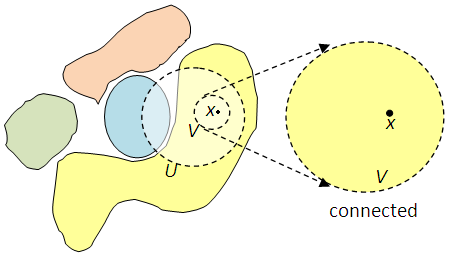
Note that since U is open in X, any subset $V\subseteq U$ is open in U if and only if it’s open in X. In such instances, we’ll sometimes abuse our language and say “V is open” without specifying the ambient space.

One useful way to judge if a space is locally connected is as follows.

Proposition 1. A topological space X is locally connected if and only if it has a basis all of whose elements are connected.

Proof.

(→) Let $U\subseteq X$ be open; we need to show it’s a union of connected open subsets of X. Indeed, for $x\in U,$ by local connectedness, there’s a connected open subset $V\subseteq U$ containing x. So U is indeed a union of connected open subsets.

(←) Let $U\subseteq X$ be open and $x\in U.$ Now we can write U as a union of connected open subsets. One of these (say V) must contain x. ♦

The key property we wish to prove is:

Theorem 2. If X is locally connected, then every connected component of X is open in X. Hence X is the topological disjoint union of its connected components.

Proof.

Let $x\in Y$ , where Y is a connected component of X. By definition, x is contained in some open connected subset U of X. Since Y is a maximal connected set containing x, we have $x\in U\subseteq Y.$ This shows that Y is open in X. ♦

Important Non-Example

Take our favourite topologist’s sine curve $X=Y\cup Z$ where:

$Y = \{0\} \times[0,1]$ and $Z=\{(x, \sin(1/x) : 0 < x\le 1\}.$

We saw that X is connected. However it is not locally-connected since for any $0 < \epsilon < 1$ , the ε-neighbourhood of the origin contains more than one (in fact infinitely many!) connected components:

This also shows that connected spaces are generally not locally connected.

Corollary. A locally connected space X is totally disconnected if and only if it’s discrete.

Proof.

If X is totally disconnected, each {x} is a connected component; since X is locally connected, each connected component is open in X. ♦

Properties of Locally Connected Spaces

Similar to the case of locally compact, the following result explains why the property is “local”.

Proposition 3. Let X be a topological space.

If $U\subseteq X$ is open, and X is locally connected, then so is U.

If $X=\cup_i U_i$ is a union of open subsets and each U_i is locally connected, then so is X.

Proof.

1st statement: let $x\in U'$ where U’ is open in U. Then U’ is open in X so there exists a connected open subset V of X such that $x\in V\subseteq U'.$ This V is also open in U.

2nd statement: let $U\subseteq X$ be open and $x\in U$ . Then $x\in U_i$ for some i. By local connectedness of U_i, and $x\in U_i\cap U \subseteq U_i,$ there exists a connected open subset V of U_i ∩ U such that $x\in V\subseteq U_i\cap U.$ Thus, $x\in V\subseteq U.$ ♦

It’s not true that if f : X → Y is continuous and X is locally connected, then so is f(X). Indeed, let X = Q with the discrete topology and Y = Q as a subspace of R. The identity map on the underlying set Q then gives a surjective continuous map but Y is not locally connected. [ Recall that if we replace “locally connected” with “connected”, then this is true. ]

Closed subsets of locally connected spaces are not locally connected in general. E.g. take X = R and $Y = \{0\} \cup \{\frac 1 n : n= 1, 2, \ldots\}.$ Then Y is closed in X, but there’s no connected open subset of 0 in Y.

–

Proposition 4. If X and Y are locally connected topological spaces, then so is X × Y.

Proof.

Since X is locally connected, there is a basis B_X comprising of open connected subsets. Likewise, pick such a basis B_Y for Y. Then $B:= \{U\times V: U\in B_X, V\in B_Y\}$ is a basis of X × Y comprising of open connected subsets. ♦

This does not hold for infinite products. For example, let X = {0, 1}^N, where {0, 1} is given the discrete topology. We claim that X is totally disconnected.

Indeed, suppose some connected component Y contains $(x_n), (y_n) \in X$ where $x_n \ne y_n$ for some n. Then projecting to the n-th component gives a surjective map $\pi_n : Y\to \{0, 1\}$ which violates the theorem that the continuous image of a connected set is connected.

Hence, X is a totally disconnected space which is not discrete (since it’s compact by Tychonoff theorem), so it can’t be locally connected (see corollary to theorem 2).

Examples

Any discrete set is locally connected since we can take V={x}.
Since the open intervals in R are connected, R has a basis of connected open subsets and is thus locally connected.
Hence Rⁿ is also locally connected by proposition 4, as is any open subset of Rⁿ by proposition 3.
Let X = [0, 1]; then X is connected and locally connected. For example, at 0, any open subset must contain $[0, \epsilon)$ for some ε>0, which is open in X.
Q is totally disconnected yet not discrete, so it’s not locally connected.

Locally Path-Connected Spaces

Correspondingly, we have locally path-connected spaces.

Definition. A topological space X is locally path-connected if

for each open subset $U\subseteq X$ and $x\in U,$ there exists a path-connected open subset V of X such that $x\in V\subseteq U.$

The earlier properties all carry over since the proofs can be replicated by replacing “path-connected” with “connected” whenever it appears in the text.

Proposition 5. A topological space X is locally path-connected if and only if it has a basis all of whose elements are connected.

Theorem 6. If X is locally path-connected, then every path-connected component of X is open in X. Hence X is the topological disjoint union of its path-connected components.

Proposition 7. Let X be a topological space.

If $U\subseteq X$ is open, and X is locally path-connected, then so is U.

If $X=\cup_i U_i$ is a union of open subsets and each U_i is locally path-connected, then so is X.

Proposition 8. If X and Y are locally path-connected, then so is X × Y.

Examples (same as earlier).

Any discrete set is locally path-connected since we can take V={x}.
Since the open intervals in R are path-connected, R has a basis of path-connected open subsets and is thus locally path-connected.
Hence Rⁿ is also locally path-connected, as is any open subset of Rⁿ.
Let X = [0, 1]; then X is path-connected and locally path-connected. For example, at 0, any open subset must contain $[0, \epsilon)$ for some ε>0, which is open in X.
Q is totally disconnected; since each connected component is a disjoint union of path components, we see that the only path components of Q are {x}. Hence, Q is not locally path-connected, for if it were, Q would have to be the disjoint union of all {x} and hence discrete.

Let’s see if we can find counter-examples similar to those for local connectedness.

Non-Properties

1. Not true: if X is path-connected, then it’s locally path-connected.

Take the circle $S^1 = \{ (x,y)\in\mathbf{R}^2 : x^2 + y^2=1\}$ and consider an infinite sequence of wheel spokes: $X_0 = [0, 1] \times \{0\}$ and:

$X_n = \{ (t\cos \frac\pi n, t\sin \frac\pi n) : \frac n {n+1}\le t\le 1\},$ for n = 1, 2, … .

Now take $X := S^1 \cup \left(\cup_{n=0}^\infty X_n\right)$ :

Now there’s no path-connected open subset V such that $(0,0)\in V\subseteq N_X((0, 0), \frac 1 2).$ On the other hand, X is clearly path-connected.

2. Not true: if f : X → Y is continuous and X is locally path-connected, then so is Y.

Same example as before: let X=Q with the discrete topology and Y=Q as a subspace of R. Then the identity map on Q is continuous and X is locally path-connected, but f(X) = Y is not.

3. Not true: a product of infinitely many locally path-connected spaces is locally path-connected.

Same example as before: X = {0, 1}^N, where {0, 1} is given the discrete topology. We saw earlier that X is totally disconnected, so the components (and hence path components) are singleton sets. On the other hand, X is not discrete, so it cannot be locally path-connected.

Relationship Between (Locally) Connected & Path-connected

Finally, let’s examine the relationship between the two notions. Since path-connected sets are connected, we have:

1. A locally path-connected space is also locally connected.

The converse isn’t true.

2. A locally connected space is not locally path-connected in general.

This is hard: one can find a counter-example in Munkres, “Topology“, 2nd edition, page 162, chapter 25, exercise 3.

3. If X is connected and locally path-connected, then it’s path-connected.

Pick any path component Y of X. Since X is locally path-connected, Y is open in X. The complement X–Y is a union of path components, each open in X, so it’s open too. Thus Y is a clopen subset of X and we must have Y=X.

Summary

The following summarises various properties of compactness, connectedness and path-connectedness. Note: for any property that mentions local compactness, we also assume X is Hausdorff.

C	Compact	Connected	Path-connected
If X is C, and f:X→Y is continuous, then f(X) is C.	🙂	🙂	🙂
If each X_i is C, then their product also is C.	🙂	🙂	🙂
C implies (locally C).	🙂	–	–
If X is locally C, then so is any open subset U of X.	🙂	🙂	🙂
If X is locally C, then so is any closed subset of X.	🙂	–	–
If $X = \cup_i U_i$ is a union of open subsets and each U_i is locally C, then so is X.	🙂	🙂	🙂
If f:X→Y is continuous and X is locally C, then so is f(X).	–	–	–
If X and Y are locally C, then so is X × Y.	🙂	🙂	🙂
If each X_i is locally C for infinitely many i, then so is their product.	–	–	–

Posted in Notes | Tagged advanced, connected components, connected spaces, locally connected, locally path-connected, path-connected components, path-connected spaces, topology, totally disconnected spaces | 4 Comments

Topology: Path-Connected Spaces

Posted on March 7, 2013 by limsup

A related notion of connectedness is this:

Definition. A path on a topological space X is a continuous map $f:[0, 1] \to X.$ The path is said to connect x and y in X if f(0)=x and f(1)=y. X is said to be path-connected if any two points can be connected by a path.

In a sense, path-connectedness is more active since one requires an explicit path to establish it, while the earlier connectedness is more passive since it simply indicates a failure to decompose as a topological disjoint union. The two are obviously related, starting from:

Theorem 1. A path-connected space X is connected.

Proof.

Suppose X is path-connected but not connected. There’s a surjective continuous map $f:X\to \{0,1\}.$ Pick $x, y\in X$ such that f(x)=0 and f(y)=1. There’s a path $g:[0, 1] \to X$ such that g(0)=x and g(1)=y. Now the composition $f\circ g:[0, 1] \to\{0,1\}$ is continuous and surjective, which contradicts the fact that [0, 1] is connected. ♦

The converse is not true: the topologist’s sine curve is connected but not path-connected. Let $X = Y\cup Z \subset \mathbf{R}^2,$ where $Y = \{0\}\times [0, 1],$ $Z=\{(x, \sin(1/x)) : 0 < x \le 1\}.$

To see why it’s not path-connected, suppose $f:[0, 1] \to X$ is continuous and f(0) = (0, 0), f(1) = (1, sin(1)).

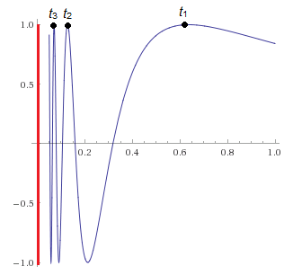
Let $\pi_x, \pi_y : X\to \mathbf{R}$ be projection maps to the x– and y-coordinates respectively. Then $\pi_x \circ f:[0, 1]\to \mathbf{R}$ contains 0 and 1, so its image is the whole [0, 1] by the intermediate value theorem. Hence, $\text{im}(f)\supset Z.$ Pick points $t_0, t_1, t_2, \ldots \in [0, 1]$ such that $f(t_n) = ((2n\pi + \frac \pi 2)^{-1}, 1).$

Since [0, 1] is compact, f is uniformly continuous. So there exists ε>0 such that whenever $t, u\in [0, 1]$ satisfy $|t-u|<\epsilon,$ we have $|\pi_y(f(t)) - \pi_y(f(u))| <1.$ Since [0, 1] is compact, we’ll pick m<n such that $|t_m - t_n|<\epsilon.$ By intermediate value theorem, there’s a point u between t_m and t_n such that $\pi_x(f(u)) = ((2m\pi + \frac {3\pi}2)^{-1}, -1).$ Then $|t_m - u| < \epsilon$ but $|\pi_y(f(t_m)) - \pi_y(f(u))| = |1-(-1)|=2>1$ which is a contradiction.

[ Notice it took quite a bit of effort to prove a seemingly obvious claim, and we needed compactness to prove it. ]

Note also that X is closed in R², and every point in Y is a point of accumulation of Z, so cl(Z) = X. In short, we have the first bummer.

Conclusion. The closure of a path-connected subset Y of X is not necessarily path-connected.

Thankfully, the next result does carry over.

Proposition 2. If $f:X\to Y$ is a continuous map of topological spaces and X is path-connected, then so is f(X).

Proof.

For any $y_0, y_1\in f(X)$ we can pick $x_0, x_1 \in X$ such that $f(x_0) = y_0, f(x_1) = y_1.$ Pick a path $f:[0, 1] \to X$ such that $f(0)=x_0$ and $f(1)=x_1.$ Then the composition gives a path $g\circ f:[0, 1] \to Y$ which connects $y_0$ to $y_1.$ ♦

Proposition 3. If $\{Y_i\}$ is a collection of path-connected subspaces of X and $\cap_i Y_i\ne\emptyset,$ then so is $Y:= \cup_i Y_i.$

Proof (Sketchy).

Pick $x\in \cap_i Y_i.$ If $y,z\in Y,$ then $y\in Y_i$ and $z\in Y_j$ for some indices i and j. Since Y_i and Y_j are path-connected and contain x, there’s a path in Y_i connecting x to y and a path in Y_j connecting x to z. Hence, concatenating gives a path connecting y to z. ♦

Proposition 4. If $\{X_i\}$ is a collection of path-connected spaces, then $X:=\prod_i X_i$ is also path-connected.

Proof.

Let $(x_i), (y_i)\in X.$ Since each $X_i$ is path connected, pick a path $f_i :[0,1]\to X_i$ such that $f_i(0) = x_i, f_i(1) = y_i.$ Now let $f:[0, 1]\to X$ be the path $f(t) := (f_i(t))_i \in X.$

To check that f is continuous, let’s use the universal property of products. It suffices to show $\pi_i \circ f : [0,1]\to X_i$ is continuous for each i, where $\pi_i :X\to X_i$ is the projection map. But $\pi_i \circ f = f_i,$ so we’re done. ♦

Note

Once again, this fails for the box topology on $\prod_i X_i.$ Since the example $\mathbf{R}^\mathbf{N}$ in the previous article is not connected, it cannot be path-connected.

Path-Connected Components

As before, we obtain the concept of path-connected components. We define, for points x, y in X, a relation x ~ y if and only if they belong to some path-connected component. Proposition 3 then tells us this gives an equivalence relation.

Definition. The equivalence classes of the above-mentioned relation are called the path-connected components.

Since a path-connected component is automatically connected, each connected component is a disjoint union of path-connected components.

Examples

It’s easy to see that any interval (closed, open or half-open) is path-connected. In particular, it’s connected.
Hence $X = [0, 1) \cup (2, 3]$ is a disjoint union of $[0, 1)$ and $(2, 3],$ each of which is a path-connected component.
The squares [0, 1] × [0, 1] and (0, 1) × (0, 1) are path-connected by proposition 4.
Consider Q as a subspace of R. Since the connected components are singleton sets, the path-connected components can’t break them down any further.
Take the topologist’s sine curve $X=Y\cup Z$ above. Y and Z are both path-connected since they’re homeomorphic to intervals. Since X is not path-connected, the path-connected components must be Y and Z. Note that Y is open while Z is closed in X. This is one example where connected components decompose further into path-connected components.

Posted in Notes | Tagged advanced, connected components, connected spaces, path-connected components, path-connected spaces, topology | 2 Comments

Topology: Connected Spaces

Posted on March 5, 2013 by limsup

Let X be a topological space. Recall that if U is a clopen (i.e. open and closed) subset of X, then X is the topological disjoint union of U and X–U. Hence, if we assume X cannot be decomposed any further, there’re no non-trivial clopen subsets of X.

Definition. The space X is connected if its only clopen subsets are X and the empty set. Equivalently, there’re no non-empty disjoint open subsets U, V of X such that $X = U\cup V.$ Otherwise, it’s disconnected.

The following characterisation of connected sets is simple but surprisingly handy.

Theorem 1. X is connected if and only if any continuous map $f:X \to \{0, 1\},$ where {0, 1} has the discrete topology, is constant.

Thus, it’s disconnected if and only if there’s a continuous surjective map $f:X \to \{0,1\}.$

Proof.

If f is not constant, then $U := f^{-1}(0)$ and $V:=f^{-1}(1)$ are non-empty disjoint open subsets such that $X=U\cup V.$ Conversely, if $X = U\cup V,$ where U, V are non-empty, disjoint and open in X, then we can set

$f:X\to \{0, 1\}, \quad x\mapsto \begin{cases} 0, &\quad\text{if } x\in U, \\ 1, &\quad\text{if } x\in V.\end{cases}$ ♦

With this theorem in hand, the remaining properties are surprisingly easy to prove.

Proposition 2. If Y is a connected subset of X, then its closure $Z := \text{cl}_X(Y)$ is connected.

Proof.

First $\text{cl}_Z(Y) = Z\cap\text{cl}_X(Y) = Z,$ so Y is dense in Z. Suppose $f:Z\to\{0, 1\}$ is continuous. Then $f|_Y$ is constant (say, 0) since Y is connected. Since $f^{-1}(0)$ is closed and contains Y, it must be the whole of Z. ♦

Proposition 3. If $f:X\to Y$ is a continuous map of topological spaces and X is connected, then so is f(X).

Proof.

Replace Y by f(X); we may assume f is surjective. Suppose $g:Y\to \{0, 1\}$ is a surjective continuous map. Then $g\circ f : X\to \{0, 1\}$ is also continuous and surjective, so X is disconnected (contradiction). Hence, g does not exist. ♦

The union of connected subsets is not connected in general; in fact, topological disjoint unions of two or more non-empty spaces are never connected. But if the spaces share a common point, we have the following.

Proposition 4. Let $\{Y_i\}$ be a collection of connected subspaces of X. If $\cap_i Y_i \ne \emptyset,$ then $Y:= \cup_i Y_i$ is connected.

Proof.

Pick $x\in \cap_i Y_i$ . Let $f:Y\to\{0, 1\}$ be a continuous map. Then each $f|_{Y_i}$ is constant for each i, and it must be equal to f(x). So f is constant. ♦

Intermediate Value Theorem

Let’s consider subsets of R. We claim:

Lemma. A subset of R is connected if and only if it’s one of the following:

bounded: $(a, b), (a, b], [a, b), [a, b]$ ;

unbounded: $(-\infty, b), (-\infty, b], (a, \infty), [a, \infty), \mathbf{R}$ ;

Proof.

The proof is long but conceptually easy. First we show that (a, b) is connected.

If not, write (a, b) as a disjoint union of non-empty open subsets U and V. Let x = sup(U) ≤ b.
Now x doesn’t lie in U. Otherwise x<b, so N(x, 2ε) lies in U for some ε>0. In particular, x+ε lies in U, so x is not an upper bound of U (contradiction).
So x lies in V. But that means for some ε>0, N(x, ε) lies in V and hence is disjoint from U. That means x-ε is an upper bound of U (contradiction).
Conclusion: (a, b) is connected.

Since (a, b) is dense in all the bounded intervals $(a, b], [a, b), [a, b],$ these are all connected by proposition 2. Finally, for the unbounded intervals, apply proposition 4. E.g. $(0, \infty) = \cup_{n=1}^\infty (0, n).$

To prove the converse, we note that if $X\subseteq \mathbf{R}$ is connected and $a,b\in X$ with a<b, then $[a,b]\subseteq X.$ [ Indeed, if a < r < b and $r\not\in X,$ then $X = ((-\infty, r)\cap X)\cup (r,\infty) \cap X)$ and the two open subsets are non-empty since they contain a and b respectively. ]

Now let b = sup(X). There’re 3 possibilities: either (i) b = ∞, (ii) b < ∞ and lies in X, or (iii) b < ∞ and doesn’t lie in X. The same holds for a = inf(X): either (a) a = -∞, (b) a > -∞ and lies in X, or (c) a > -∞ and doesn’t lie in X. Each of the 9 possibilities gives rise to an interval above. We’ll leave the details to the reader.

[ Example for case (i)(b). For each x>a, x is not a lower bound of X so there exists y<x, y lies in X. Since sup(X) = ∞, there exists z>x which lies in X. So $[y,z]\subseteq X$ and $x\in X.$ Thus, $(a,\infty) \subseteq X.$ The fact that a isn’t in X shows that equality holds. ] ♦

Corollary (Intermediate Value Theorem). If $f:[a,b]\to \mathbf{R}$ is continuous, then the image of f is also a closed interval [c, d]. In particular, if s lies between f(a) and f(b), then there exists an r in [a, b], f(r) = s.

Proof.

Since [a, b] is a compact and connected subset of R, so is f([a, b]). Out of the 9 possible connected subsets of R, only the closed interval [c, d] is closed and bounded. Thus, f([a, b]) = [c, d]. ♦

Connected Components

Let X be a topological space. For any two points x, y in X, write x ~ y if there’s a connected subset of X containing them. We claim this gives an equivalence relation; indeed, it is clearly reflexive and symmetry. Transitivity follows straight from proposition 3.

Definition. The equivalence classes of this relation are called the connected components of X.

Note that each connected component Y is a maximal connected subset of X, in the sense that if we add any point outside Y, the resulting set won’t be connected.

We know that X is a set-theoretic disjoint union of its connected components. It’s tempting to think that X is a topological disjoint union as well. But that’s wrong. Indeed, let’s look at X = Q (as a subspace of R). The only connected subsets of X are the singleton points {x}: for if $Y\subseteq X$ and $a,b\in Y$ with a<b, then we can pick an irrational r, a<r<b so that $Y = ((-\infty, r)\cap Y) \cup ((r, +\infty)\cap Y)$ is a disjoint union of two non-empty open subsets. So Y is disconnected.

Thus, the connected components of Q are the singleton sets. But Q is clearly not discrete.

Definition. A space whose connected components are all singleton sets is said to be totally disconnected.

Thus, a discrete space is totally disconnected but not vice versa.

The example of Q shows that connected components are in general not open. However, they’re closed.

Proposition 5. Every connected component Y of a topological space X is closed.

Proof.

This follows almost immediately from proposition 2: since Y is connected, so is $\text{cl}_X(Y)\supseteq Y.$ But Y is a maximal connected subset, so $Y = \text{cl}_X(Y).$ ♦

Proposition 6. If $\{X_i\}$ is a collection of non-empty topological spaces, the product $X := \prod_i X_i$ is connected if and only if each $X_i$ is connected.

Proof.

(→) is obvious since each $X_i$ is the continuous image of the projection map from X. For (←), let $f:X\to \{0,1\}$ be surjective and continuous. Let $(x_i)\in f^{-1}(0).$ Since $f^{-1}(0)$ is open, it contains a basic open set of the form $\prod_i U_i$ where $U_i=X_i$ for all but finitely many i‘s : $\{i_1, \ldots, i_n\}.$ Thus:

$\left(\prod_{i\ne i_1,\ldots, i_n} X_i\right) \times \{x_{i_1}\} \times \{x_{i_2}\} \times\ldots\times \{x_{i_n}\} \subseteq f^{-1}(0).$ (#)

Next, use the following.

Sublemma. If j is an index, and $(x_i), (y_i) \in X$ satisfy: $x_i = y_i$ for all i except i=j, then they belong to the same connected component.
Proof. The subspace $X_j \times (\prod_{i\ne j} \{x_i\})$ is homeomorphic to X_j so it is a connected subset containing $(x_i), (y_i).$

Hence on the LHS of (#), we can change the coordinates $x_{i_1}, \ldots, x_{i_n}$ one at a time and see that the whole $\prod_i X_i$ is contained in $f^{-1}(0),$ i.e. X is connected. ♦

The above sublemma holds for the box topology too. This may con us into believing that $\prod_i X_i$ under the box topology is also connected. But let’s take $X=\mathbf{R}^\mathbf{N},$ the space of all real sequences and U the subset of all sequences converging to 0. Any $(x_n) \in U$ is also contained in $\prod_{n=1}^\infty (x_n - \frac 1 n, x_n + \frac 1 n)$ which is open in the box topology and contained in U. Thus U is open. The same holds for any $(x_n)\in X-U$ so X–U is also open. [ Note that the sublemma implies altering a single term in a sequence has no effect on whether it converges to 0. ]

Examples

An infinite set with the cofinite topology is connected since all non-empty closed subsets are finite and hence not open.
The space $X = [0, 1)\cup (2, 3]$ is disconnected since $[0, 1) = (-1, 1) \cap X$ and $(2, 3] = (2, 4)\cap X$ are open subsets of X. These give the connected components of X.
By proposition 6, the square [0, 1] × [0, 1] is connected, as is its interior (0, 1) × (0, 1) in R².
The circle S¹ is connected since it’s the continuous image of $t\mapsto (\cos(t),\sin(t)).$
(Topologist’s Sine Curve) Take the set $X = Y\cup Z \subset \mathbf{R}^2,$ where $Y = \{0\}\times [0, 1],$ $Z=\{(x, \sin(1/x)) : 0 < x \le 1\}.$ Now Y and Z are homeomorphic to [0, 1] and (0, 1] respectively, so they’re connected. What’s surprising is that X is connected as well! Indeed, one observes that Y is a set of accumulation points for Z, since for every open point (0, y) in Y and ε>0, $N_X((0, y), \epsilon)$ contains a point of Z. Thus $\text{cl}_X(Z) = X.$ Since Z is connected, proposition 2 tells us X is connected too.

Exercise.

Which of the following is/are correct for a subset Y of X?

If cl(Y) is connected, then so is Y.
If Y is connected, then so is int(Y).
If int(Y) is connected, then so is Y.

Answer (Highlight to Read).

They’re all wrong! First statement: let X = R and Y be the union of (-1, 0) and (0, 1); cl(Y) = [-1, 1]. Second statement: let X = R² and Y be the union of [-1, 0] × [-1, 0] and [0, 1] × [0, 1]. Each square is connected; since they share a common point, Y is connected. But int(Y) is the disjoint union of two open squares. Third statement: let Y be {0, 1} in R; int(Y) is empty and hence connected. ♦

Posted in Notes | Tagged advanced, box topology, connected components, connected spaces, intermediate value theorem, product topology, topology, totally disconnected spaces | Leave a comment

Topology: One-Point Compactification and Locally Compact Spaces

Posted on March 3, 2013 by limsup

Compactifications

There’re lots of similarities between completeness and compactness, beyond the superficial resemblance of the words. For example, a closed subset of a compact (resp. complete) space is also compact (resp. complete). Two differences though:

compactness is a topological concept while completeness depends on the underlying metric;
compact metric spaces are complete (proposition 4 here) but not vice versa.

[ Intuitively, complete metric spaces can become unbounded and thus fail to be compact. But merely boundedness is not enough to ensure compactness, since any metric can be massaged to a bounded one without affecting the underlying topology. Indeed, it turns out a metric space is compact if and only if it’s complete and totally bounded. We won’t prove that here, but the interested reader may attempt it (it’s not too hard). ]

Also, any metric space can be “filled out” to give a completion. Likewise, can we compactify a general topological space?

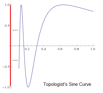
Definition. A compactification of a topological space X is a compact space Y containing X, such that $X\hookrightarrow Y$ is a dense subspace of Y.

Upon doing that, we immediately run into the problem of uniqueness, i.e. the completion is unique while the compactification isn’t. E.g. (0, 1) can be compactified to give both [0, 1] and the unit circle $S^1 := \{(x,y)\in\mathbf{R}^2 : x^2 + y^2 = 1\}.$

Nonetheless, let’s continue exploring compactifications. The easiest way is to add just one point.

One-Point Compactifications

Task. Given a topological space X, we wish to construct a compact space Y by appending one point: $Y = X \cup \{\infty\}.$ This is called a one-point compactification of X.

Examples.

A one-point compactification of (0, 1) (or R) is given by the circle $S^1 := \{ (x,y)\in\mathbf{R}^2 : x^2+y^2=1\}$ in the plane.
A one-point compactification of [0, 1) is given by [0, 1].
A one-point compactification of $(0, 1) \cup (2, 3)$ is given by the union of two circles which are tangent to each other.
A one-point compactification of the plane R² is given by the 2-sphere $\{(x,y,z)\in\mathbf{R}^3 : x^2+y^2+z^2=1\}$ in 3-space.

Describing the Topology of Y

What would the topology of Y look like? We’ll start by making a reasonable assumption: that X is open in Y (i.e. {∞} is closed in Y). Now, given any open subset V of Y.

If $\infty\not\in V,$ then V is an open subset of Y contained in X, so V is open in X.
If $\infty\in V$ , then C := Y–V is closed in X. Also C is compact since it’s a closed subset of the compact space Y.

This inspires us to define open subsets of Y as follows:

not containing ∞: open subsets U of X, or
containing ∞: sets Y–C, where C is a closed subset of X which is compact.

Checking that this gives us a topology.

Indeed, a union of sets of the first type is of the first type.
A union of sets of the second type $\cup_i (Y-C_i) = Y-\cap_i C_i$ is of the second type (it’s compact since ∩C_i is closed is closed in each C_i).
Finally, $U\cup (Y-C) = Y-(C\cap (X-U))$ and C ∩ (X–U) is closed in X and compact since it’s a closed subset of C.

Obviously, X is open in Y and has the subspace topology.

Showing that Y is compact.

Let $Y = (\cup_i U_i) \cup (\cup_j (Y-C_j))$ be an open cover. Then there’s at least one C_j, and

$C_j \subseteq (\cup_i U_i) \cup (\cup_{j'\ne j} (Y-C_{j'})).$

Since C_j is compact, it has a finite subcover. Together with Y–C_j, this forms a finite subcover of Y.

Definition. The above construction is called the Alexandroff extension of the space X. It extends X by one point to give a compact space Y.

Examples and Properties

Suppose X = (0, 1). We map its Alexandroff extension $f:Y\to S^1$ by $t\mapsto (\cos(2\pi t), \sin(2\pi t))$ and $\infty \mapsto (1, 0).$ Clearly f is continuous outside ∞. For continuity at ∞, an open subset containing (1, 0) must contain the set V of $(\cos(2\pi t), \sin(2\pi t)),$ $-\epsilon<t<\epsilon,$ for some ε>0. Then $f^{-1}(V)$ is the set $Y - [\epsilon, 1-\epsilon]$ which is open in the Alexandroff extension. Now we’ll finish the proof by a trick.

Lemma. If X is a compact space, Y is Hausdorff, and $f:X\to Y$ is a bijective continuous map, then f is a homeomorphism.

Proof.

Continuity means $f^{-1}$ maps closed subsets to closed subsets. It suffices to show f maps closed subsets to closed subsets. But if C is closed in X, then C is compact and thus f(C) is compact. Since Y is Hausdorff, f(C) is closed in Y. Done. ♦

Let’s take the second example $X=[0,1)$ . Map the Alexandroff extension $f:Y \to [0,1]$ by taking t to itself and ∞ to 1. Once again f is continuous outside ∞. For continuity at ∞, an open subset containing 1 in [0, 1] must also contain V = (1-ε, 1] for some ε>0. But then $f^{-1}(V) = Y - [0, 1-\epsilon]$ which is open in the Alexandroff extension. Hence f is continuous and we invoke the above lemma to show that it is a homeomorphism.
Let X = Q. Then Y is not Hausdorff since there’re no disjoint open subsets U and V separating 0 and ∞. To see why, replacing an open subset by a smaller one, we may take $U=(-\epsilon, +\epsilon)\cap \mathbf{Q}$ containing 0. For ∞, we have V = Y–C, for a compact subset C of Q containing U. This means $[-\epsilon, +\epsilon] \cap\mathbf{Q}$ is closed in C and hence also compact, which is impossible by this lemma.

Lemma. The subspace $C:=[a, b] \cap \mathbf{Q}\subset \mathbf{R}$ for a<b is not compact.

Proof.

Indeed, C is not closed in R since its complement Y := R–C contains an irrational r, a<r<b, and no open neighbourhood of r is contained in Y. ♦

Now we’ll state some properties of the Alexandroff extension Y of X.

Property 1. X is dense in Y if and only if X is not compact.

Proof.

The closure of X in Y is either X or Y. Thus, X is not dense in Y iff X is closed in Y iff {∞} is open in Y iff X = Y-{∞} is compact. ♦

Property 2. Y is Hausdorff if and only if X is Hausdorff, and every $x\in X$ is contained in an open subset U such that $\text{cl}_X(U)$ is compact.

Proof.

(→) : every subspace of a Hausdorff space is Hausdorff. To show X is locally compact, let $x\in X.$ Pick open subsets U, V of Y such that $x\in U, \infty\in V, U\cap V=\emptyset.$ Now V = Y–C for some closed compact subset C of X. Then $x\in U\subseteq C.$ Since cl_X(U) is closed in C, it’s compact.

(←) : since X is open in Y, any two points in $X\subseteq Y$ can be separated by open subsets. The only problem is $x\in X, y = \infty\in Y.$ Pick open subset U of X containing x such that C := cl_X(U) is compact. Then U and Y–C are open subsets of Y which separate x and y. ♦

Finally, we end this section with an exercise.

Exercise.

Prove that if Y, Y’ are the Alexandroff extensions of X, X’ respectively, and f : X → X’ is continuous, then the map g : Y → Y’ which takes an element x of X to f(x) and ∞ to ∞ is also continuous.

Answer.

Since X is open in Y and f is continuous, g is also continuous on X. It remains to check ∞. Let V = Y’ – D be an open subset of Y’ where D is a closed compact subset of X’. Now f-1(V) = X’ – f-1(D), where C := f-1(D) is closed in X.

Locally Compact Spaces

The following definition is inspired by the above results.

Definition. A topological space X is said to be locally compact if for each $x\in X,$ there’s an open subset U containing x such that cl(U) is compact.

For example, compact spaces are clearly locally compact. Our discussion above tells us:

One-Point Compactification Theorem. If X is a Hausdorff and locally compact space which is not compact, then the Alexandroff extension Y is the unique one-point compactification of X which is Hausdorff.

The following alternative definition of local compactness is rather common.

Theorem 1. If X is Hausdorff, then it is locally compact if and only if for any $x\in X$ and open subset U containing x, there’s an open subset V containing x such that

$x\in V\subseteq \text{cl}(V) \subseteq U$

and cl(V) is compact.

Proof.

(←) is obvious. For (→), let U be an open subset of X containing x. Pick open V containing x such that cl(V) is compact. Let C = cl(V)-U = cl(V) ∩ (X–U), which is closed in cl(V) and hence compact. For each $y\in C,$ separate x and y by open subsets $W_y, W_y'$ such that

$x\in W_y,\ y\in W_y', \ W_y \cap W_y'=\emptyset.$

Since $\cup_{y\in C} W_y' \supseteq C$ and C is compact, there’s a finite set of points $y_1, y_2, \ldots, y_n$ such that $W' := \cup_{i=1}^n W_{y_i}' \supseteq C.$ Let $W = U\cap V\cap (\cap_{i=1}^n W_{y_i})$ which gives an open subset containing x which doesn’t intersect W’. Thus, cl(W) also doesn’t intersect W’, and $\text{cl}(W) \subseteq \text{cl}(V) - C \subseteq U$ :

$x\in W \subseteq \text{cl}(W) \subseteq U$ , with cl(W) closed in cl(V) and hence compact. ♦

If X is not Hausdorff, then this theorem fails. E.g. example 3 above (Alexandroff extension Y of Q) is compact, and hence locally compact by our definition. Yet the open subset $(-1, 1)\cap\mathbf{Q}$ of Y doesn’t contain an open subset whose closure in Y is compact. This is because any such open subset contains $(a,b)\cap\mathbf{Q}$ and the closure thus contains $[a,b]\cap \mathbf{Q}$ so this $[a,b]\cap \mathbf{Q}$ must be compact (impossible).

Hence, we’ll only consider locally compact spaces which are also Hausdorff. Note that a locally compact metric space is not necessarily complete, e.g. (0, 1) is a counter-example.

Properties of Locally Compact Spaces

The following result explains why the property is “local”.

Theorem 2. Let X be a Hausdorff space.

If X is locally compact, then so is any open subset U.

If $X = \cup_i U_i$ is an open cover of X and each U_i is locally compact, then so is X. In particular, a disjoint union of locally compact spaces is locally compact.

Proof.

[ Note: throughout the proof, be careful when talking about open and closed subsets, since we’ve to specify the ambient space too. ]

1st statement: if U’ is an open subset of U containing x, then it’s also an open subset of X containing x. By theorem 1, there’s an open subset V of X such that $x\in V\subseteq \text{cl}_X(V) \subseteq U',$ where cl_X(V) is compact. Since V is an open subset of X contained in U, it’s also open in U; also $\text{cl}_U(V) =\text{cl}_X(V) \cap U = \text{cl}_X(V).$

2nd statement: if U is an open subset of X containing x, pick any i such that $x\in U_i.$ By theorem 1, there exists V (open in U_i and hence in X) containing x such that $x\in V\subseteq \text{cl}_{U_i}(V) \subseteq U\cap U_i$ and $\text{cl}_{U_i}(V)$ is compact and hence closed in X. Thus $\text{cl}_X(V) \subseteq\text{cl}_{U_i}(V)$ and conversely, $\text{cl}_{U_i}(V) = \text{cl}_X(V) \cap U_i \subseteq \text{cl}_X(V).$ So $x\in V\subseteq \text{cl}_X(V) \subseteq U$ and cl_X(V) is compact. ♦

Exercise.

Prove that if X is locally compact and Hausdorff, then so is any closed subset $C\subseteq X.$

Answer (Highlight to read).

Let U be an open subset of C containing x; write U = U’ ∩ C for some open subset U’ of X. By theorem 1, there’s an open subset V’ of X, containing x, such that its closure cl_X(V’) is compact and contained in U’. The open subset V = V’ ∩ C of C then contains x, and its closure cl_C(V’) = cl_X(V’) ∩ C is closed in cl_X(V’) and hence compact. ♦

Theorem 3. If X and Y are locally compact and Hausdorff, so is X × Y.

Proof.

Let $(x, y) \in X\times Y$ . By local compactness of X, there’s an open subset U of X containing x such that $\text{cl}_X(U)$ is compact. Likewise, there’s an open subset V of Y containing y such that $\text{cl}_Y(V)$ is compact. Thus, (x, y) is contained in U × V, whose closure $\text{cl}(U\times V) = \text{cl}(U)\times \text{cl}(V)$ is compact. ♦

The product of infinitely many locally compact spaces is not locally compact in general (to get a locally compact space, one uses the restricted product which leads to adeles and ideles in algebraic number theory). E.g., let X = R^I, where I is infinite. Then any non-empty open subset U of X contains a basic open set of the form $\prod_{i\in I} U_i,$ where each $U_i\subseteq \mathbf{R}$ is open and equality holds for all but finitely many i. The same must hold for any open $V\subseteq U$ and cl(V) can’t be compact since projecting it onto one of the coordinates covers the whole R.

Examples

Any discrete topological space is locally compact and Hausdorff.
R is locally compact since if U contains x, then it must contain some (x-2ε, x+2ε) for some ε>0. Thus U contains (x-ε, x+ε) and its closure [x-ε, x+ε] which is compact.
Thus, Rⁿ is locally compact, and so is any open or closed subset of Rⁿ.
The set X = {1/n : n = 1, 2, 3, … } is locally compact since it’s discrete. Its closure, given by $X\cup \{0\}$ , is in fact compact.
The set of rationals Q is not locally compact since it’s Hausdorff but its Alexandroff extension is not.

Exercise

Is it true that if f : X → Y is continuous and X is locally compact, then so is Y? [ Recall that this is true if we replace “locally compact” by “compact”. ]

Answer (Highlight to read)

No, take X = Q with the discrete topology and Y = Q as a subspace of R. Then the identity map f : X → Y is continuous but Y = f(X) is not locally compact. ♦

Posted in Notes | Tagged advanced, Alexandroff extensions, compact spaces, compactifications, Hausdorff, locally compact spaces, one-point compactification, topology | 6 Comments

Topology: Finite Intersection Property (Omake)

Posted on February 28, 2013 by limsup

The whole point of this article is the following seemingly trivial observation.

Theorem. A topological space X is compact if and only if it satisfies the finite intersection property (F.I.P.):

if $\{C_i\}$ is a collection of closed subsets of X such that every finite intersection $C_{i_1} \cap C_{i_2} \cap\ldots \cap C_{i_n}\ne\emptyset,$ then $\cap_i C_i\ne\emptyset.$

Proof.

Suppose X is compact. Then given a collection {C_i} of closed subsets of X with empty intersection, we have $\cup_i (X-C_i) = X - \cap_i C_i = X$ so the open cover {X–C_i} has a finite subcover. This gives a finite collection of C_i with empty intersection.

The converse is just as easy: if F.I.P. holds and $\{U_i\}$ is an open cover of X, then $\cup_i U_i = X\implies \cap_i (X-U_i) = \emptyset.$ By F.I.P., there’s a finite collection $(X-U_{i_1}) \cap \ldots\cap (X-U_{i_n})=\emptyset$ so $\cup_n U_{i_n} = X$ is a finite subcover. ♦

Though this looks like a simple rephrasing of the definition of compact spaces, its underlying philosophy embodies an entire paradigm shift. [ Ok, that’s probably stretching it a little … ] The idea is that a closed subset of X typically represents a subset which satisfies certain nice conditions. Hence F.I.P. means that if every finite set of conditions can be satisfied by some object, then there’s some object that satisfies all conditions.

To make it a little more explicit, let’s prove the following.

Proposition. Suppose $X_0, X_1, X_2,\ldots$ are non-empty compact Hausdorff spaces and $f_n : X_n \to X_{n-1}$ is a collection of continuous maps:

$\ldots \stackrel{f_{n+1}}\longrightarrow X_n \stackrel{f_n}\longrightarrow X_{n-1} \stackrel{f_{n-1}}\longrightarrow \cdots \stackrel{f_2}\longrightarrow X_1 \stackrel{f_1}\longrightarrow X_0.$

Then there exists a sequence $(\ldots, x_n, \ldots, x_2, x_1, x_0),$ where $x_n \in X_n$ and $f_n(x_n) = x_{n-1}$ for each n≥1.

Compactness is essential here. For example, if $X_n = (0, \frac 1 n)$ and each f_n is the inclusion map, then no such sequence exists since the intersection of all X>n is empty.

Proof.

Let $X = \prod_{i=0}^\infty X_i$ which is compact by Tychonoff’s theorem. For each n≥1, let:

$C_n = \{ (\ldots, x_2, x_1, x_0)\in X : f_i(x_i) = x_{i=1} \text{ for } 1\le i\le n\}.$

Note that $C_1 \supseteq C_2 \supseteq C_3 \supseteq \ldots .$ Also $C_n$ is homeomorphic to $Y_n := \prod_{i=n}^\infty X_i$ via the following mutually inverse maps:

$\begin{aligned} C_n \to Y_n, &\quad (\ldots, x_n, \ldots, x_2, x_1, x_0)\mapsto (\ldots, x_n)\\ Y_n\to C_n, &\quad (\ldots, x_n) \mapsto (\ldots, x_n, f_n(x_n), f_{n-1}(f_n(x_n)), \ldots, f_1 (\ldots (f_n(x_n)))\ ).\end{aligned}$

Thus $C_n$ is non-empty and compact. Since X is Hausdorff, $C_n$ is closed in X. By F.I.P., $\cap_{n=1}^\infty C_n \ne\emptyset.$ ♦

In particular, if X_n is finite with the discrete topology, then it’s compact Hausdorff and any map f_n is continuous.

Corollary. If $X_0, X_1, \ldots$ is a sequence of non-empty finite sets and $f_n : X_n \to X_{n-1}$ is a collection of functions, then we can find $(\ldots, x_2, x_1, x_0)\in \prod_n X_n$ such that $f_n(x_n) = x_{n-1}$ for each n≥1.

Once again, a deceptively simple result. It looks obvious until one really attempts to prove it. [ Try proving it directly; bear in mind f_n is not surjective in general. ]

Application: Infinite Four-Colour Theorem

We know the four-colour theorem for maps with finitely many countries, namely, any such map can be coloured by at most four colours such that no two countries which share a border have the same colour.

What about a map with countably infinite number of regions? It’s not entirely clear that four colours suffice. One may be inclined to reason as follows: start with a region with finitely many countries – we know this can be coloured by four colours – then extend the colouring to other countries one at a time. The problem with this approach is that if we start with a bad colouring, then we may get stuck and be forced to retrace the steps, and how do we prove that retracing the steps must eventually lead to a valid colouring?

Compactness to the rescue.

Label each country as 1, 2, 3, … . Let X_n be the set of colourings of the map restricted to countries 1, …, n, with 4 colours such that two countries which share a border do not have the same colour. We have a map $f_n : X_n \to X_{n-1}$ by ignoring the colour of the n-th country.

Now, classical four-colour theorem tells us each X_n is non-empty. So by the above corollary, there’s a sequence $(\ldots, x_2, x_1, x_0)$ with $x_n \in X$ such that $f_n(x_n) = x_{n-1}$ for each n. This corresponds to a colouring for the entire infinite map. ♦

Application: Infinite Tiling

Suppose we wish to fit a countably infinite set of shapes in a bounded region.

Now we assume that every finite subset of shapes can be fitted within the bounded region without overlaps. [ We say that two shapes overlap if their interiors share a common point. Also a shape is within the bounded region as long as its interior is inside. ]

Claim. Under this assumption, the entire infinite class of shapes can be placed in the region without overlaps.

Proof.

Label the shapes by 1, 2, 3, … . For each n, let X_n be the set of ways to fit shapes 1 to n within the region. The map $f_n : X_n \to X_{n-1}$ is given by removing shape n.

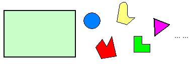
The placement of each shape i can be parametrised by coordinates $(x_i, y_i)$ and a point on the unit circle representing its orientation. Thus X_n can be parametrised by 2n coordinates and n points on the unit circle, which forms a subset of R⁴ⁿ. This subset is clearly bounded; it’s also closed because its complement is open: e. g. if two shapes have overlapping interiors, then by perturbing all shapes a little, those two shapes still overlap. Thus, by the Heine-Borel theorem, X_n is compact. The above proposition tells us there’s a way to fit all shapes in. ♦

Note

Suppose we change the condition of overlap just a little: now two shapes are said to overlap if there’s a common point (even at the boundary). Then consider rectangles 1 × 2^–n, for n = 1, 2, 3, … , to be packed in the square 1 × 1. Since $\sum_{n=1}^\infty 2^{-n} = 1,$ there’s a way to pack every finite set of rectangles in the square, but if we attempt to pack the entire infinite set, some of them must share an edge and thus overlap.

Posted in Notes | Tagged advanced, compact spaces, finite intersection property, four colour theorem, topology | Leave a comment

Topology: More on Compact Spaces

Posted on February 26, 2013 by limsup

In the previous article, we defined compact spaces as those where every open cover has a finite subcover, i.e. if $X = \cup_i U_i,$ then we can find a finite set of indices $i_1, i_2, \ldots, i_n$ such that $X = \cup_{k=1}^n U_{i_k}.$ On an intuitive level, one should imagine a compact space as being constrained, and is the topological equivalent of a finite set.

We also showed that in the case of metric spaces, compactness is equivalent to sequential compactness. Thus, the two concepts are very similar. In fact, we’ll see a parallel between the properties of compact spaces and the corresponding properties of sequentially compact spaces.

First, a simple result:

Lemma. A subspace $Y\subseteq X$ is compact if and only if :

for any collection of open subsets $\{U_i\}$ of X such that $\cup_i U_i \supseteq Y,$ there exists a finite set of indices $i_1, i_2, \ldots, i_n$ such that $\cup_{k=1}^n U_{i_k}\supseteq Y.$

Proof

(→) : Y is compact. If $\cup_i U_i\supseteq Y$ we have $\cup_i (U_i\cap Y) = Y$ and each $U_i\cap Y$ is open in Y. Thus, there’s a finite subcover $\cup_{k=1}^n (U_{i_k}\cap Y) = Y$ which gives $\cup_{k=1}^n U_{i_k} \supseteq Y.$

(←) : let $\{V_i\}$ be an open cover of Y. Each $V_i = U_i\cap Y$ for some open subset U_i of X. Now $\cup_i V_i = Y \implies \cup_i U_i \supseteq Y.$ By assumption, there’s a finite set of indices $i_1, \ldots, i_n$ such that $\cup_{k=1}^n U_{i_k}\supseteq Y$ which gives $\cup_{k=1}^n V_{i_k}=Y.$ ♦

Thus, $Y\subseteq X$ is compact if and only if every open cover of Y has a finite subcover, where “open cover” means a collection of open subsets of X whose union contains Y.

Properties of Compact Spaces

Next, we have:

Proposition 1.

If Y is a closed subset of compact space X, then Y is compact.

If Y is a compact subset of Hausdorff space X, then Y is closed in X.

Proof

1st statement: suppose $\{U_i\}$ is a collection of open subsets of X such that $\cup_i U_i\supseteq Y.$ Then $\{U_i\}$ together with X–Y is an open cover of X. Hence, there’s a finite subcover of X:

$U_{i_1}\cup U_{i_2}\cup \ldots \cup U_{i_n} \cup (X-Y) = X \implies \cup_{k=1}^n U_{i_k} \supseteq Y.$

By the lemma, Y is compact.

2nd statement: suppose x is a point of accumulation of Y and $x\not\in Y$ .

For each y in Y, separate x and y by open subsets of X: $x\in U_y, y\in V_y, U_y\cap V_y=\emptyset.$
Since $Y \supseteq \cup_{y\in Y} V_y$ and Y is compact, we can find a finite subcover: $Y \supseteq \cup_{k=1}^n V_{y_k}.$
Let $U = \cap_{k=1}^n U_{y_k}$ which is open in X and contains x. Since $U_{y_k}\cap V_{y_k} = \emptyset$ for each k, we have $U\cap Y=\emptyset,$ which contradicts the fact that x is a point of accumulation of Y. ♦

Note

Counter-examples exist for the second statement if X is not Hausdorff. E.g. if X = {1, 2} with the coarsest topology and Y = {1}, then Y is compact but not closed in X.

Proposition 2. If f : X → Y is a continuous map and X is compact, then f(X) is compact.

Proof.

Let $\{V_i\}$ be a collection of open subsets of Y such that $\cup_i V_i \supseteq f(X).$ Letting $U_i = f^{-1}(V_i),$ we have

$\cup_i U_i = \cup_i f^{-1}(V_i) = f^{-1}(\cup_i V_i) = X.$

Thus, there’s a finite subcover $\cup_{k=1}^n U_{i_k} = X$ which gives $\cup_{k=1}^n V_{i_k} \supseteq f(X).$ By the above lemma, f(X) is compact. ♦

Proposition 3. If $Y, Z\subseteq X$ are compact, then so is $Y\cup Z.$ Thus a finite union of compact subspaces is compact.

Proof.

Let $\{U_i\}$ be an open cover for $Y\cup Z.$ Then since $\cup_i U_i \supseteq Y$ and Y is compact, there’s a finite set of indices $i_1, \ldots, i_n$ such that $\cup_{k=1}^n U_{i_k} \supseteq Y.$ Likewise, there’re indices $i_{n+1}, \ldots, i_m$ such that $\cup_{k=n+1}^m U_{i_k} \supseteq Z.$ Then $\cup_{k=1}^m U_{i_k} = Y\cup Z$ so $\{U_i\}$ has a finite subcover. ♦

It’s also true that a product of compact spaces is compact. In the case of finite products, the proof isn’t hard, but what we’d like to show is the case of arbitrary products. Known as Tychonoff’s theorem, its proof is tricky and we’ll leave it till later. For now the reader may try to prove as an exercise that if X and Y are compact, then so is X × Y.

Proposition 4. A compact metric space X is complete.

Proof.

X is sequentially compact. Thus, a Cauchy sequence $(x_n)$ in X must have a subsequence which converges to a in X. Since $(x_n)$ is Cauchy, this implies $(x_n)\to a.$ ♦

Note.

Clearly compactness is a stronger condition than completeness. E.g. R is complete but not compact. On an intuitive level, completeness says “if a sequence of points get successively closer, they must converge” while compactness says “in every sequence, some of the points must converge”.

Heine-Borel Theorem. A subspace X of R is compact if and only if it’s closed in R and bounded.

Proof.

Since X is a metric space, it is compact iff it’s sequentially compact. And by corollary 4 of previous article, this is true iff X is closed in R and bounded. ♦

Finally for metric spaces, we have:

Theorem. If f : (X, d) → (Y, d’) is a continuous map of metric spaces and X is compact, then f is uniformly continuous.

Proof.

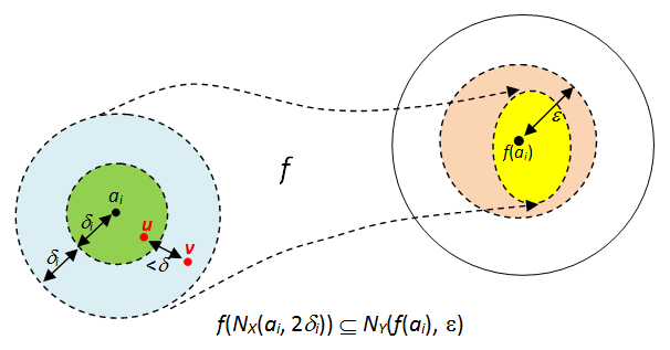
Let ε>0. For each $a\in X$ , continuity at a means there’s a δ>0 such that $f(N_X(a, 2\delta)) \subseteq N_Y(f(a), \epsilon).$ Now the collection of the open balls $N_X(a, \delta)$ covers X, so it has a finite subcover

$X = N_X(a_1, \delta_1) \cup\ldots \cup N_X(a_n, \delta_n),$ where $f(N_X(a_i, 2\delta_i))\subseteq N_Y(f(a),\epsilon).$

Let $\delta = \min(\delta_i).$ Now whenever $d_X(u, v) <\delta,$

$u\in N_X(a_i, \delta_i)$ for some 1 ≤ i ≤ n;
then $d_X(a_i ,v) \le d_X(a_i, u) + d_X(u, v) < \delta_i + \delta \le 2\delta_i$ ;
thus $d_Y(f(a_i), f(u)) < \epsilon$ and $d_Y(f(a_i), f(v)) < \epsilon$ ;
so $d_Y(f(u), f(v)) < 2\epsilon.$

And we’re done. ♦

Alexander’s Subbase Theorem

If we fix a basis B of a given topological space X, in determining whether every open cover of X has a finite subcover, we may assume this cover is from B.

Proposition 5. X is compact if and only if:

any collection of basic open sets $\{V_i\}\subseteq B$ which covers X, has a finite subcover.

Proof.

Suppose the given condition holds. To prove compactness, let {U_i} be an open cover of X. Write each $U_i = \cup_j V_{ij}$ as a union of basic open sets $V_{ij}\in B.$ Then $X = \cup_{i,j} V_{ij}$ and there must be a finite subcover

$X = V_{i_1 j_1} \cup V_{i_2 j_2} \cup \ldots \cup V_{i_n j_n}.$

Since $V_{i_k j_k}\subseteq U_{i_k}$ we have $X = \cup_{k=1}^n U_{i_k}.$ ♦

Alexander’s subbase theorem says we can push this to the level of a subbasis!

Alexander’s Subbase Theorem. If S is a subbasis of X, then X is compact if and only if:

any collection of subbasic open sets $\{W_j\} \subseteq S$ which covers X, has a finite subcover.

Proof.

The proof relies on a non-trivial set-theoretic result known as Zorn’s lemma. Let B be the basis obtained from taking finite intersections of elements from S. If X is not compact, by proposition 5, there’s a collection $\Sigma := \{V_i\} \subseteq B$ of basic open sets which covers X but with no finite subcover. We’ll assume Σ is “maximal”, i.e.

Σ has no finite subcover, but for any $V\in B-\Sigma,$ the collection $\Sigma\cup \{V\}$ has a finite subcover, which must include V. [ Note: we don’t assume there’s a unique maximal Σ. ]

We’ll defer its discussion till later and urge the reader to just accept it for now. Maximality of Σ then implies:

If $V_1, \ldots, V_n\in B$ satisfy $V_1\cap \ldots\cap V_n\in \Sigma,$ then we have $V_i\in \Sigma$ for some i. [ Indeed, if each $V_i\in B-\Sigma,$ then maximality implies $\Sigma\cup \{V_i\}$ has a finite subcover, say $X = (\cup_j V_{ij}) \cup V_i$ where each $V_{ij} \in \Sigma.$ Then $X = (\cup_{i, j} V_{ij})\cup V$ is a finite subcover of Σ. Contradiction. ]

Now we claim that Σ ∩ S covers X. For if $x\in X,$ we can find a $V\in\Sigma$ such that $x\in V.$ Since V is a basic open set, write $V = W_1\cap \ldots \cap W_n$ for $W_i\in S.$ The above condition then implies $W_i\in \Sigma$ for some i. Since $x\in W_i,$ we see that

$X = \cup_{W\in \Sigma\cap S} W,$

By the given condition, Σ ∩ S has a finite subcover, so Σ has a finite subcover, which is a contradiction. ♦

Corollary (Tychonoff’s Theorem). If $\{X_i\}$ is a collection of compact spaces, then $X:=\prod_i X_i$ is compact.

Proof.

For index i and open subset $U_i\subseteq X_i,$ the collection of open slices $V_i := (\prod_{j\ne i} X_j) \times U_i$ forms a subbasis for X. Suppose we have an open cover of X of the form {V_i}. Then for some index i, the union of U_i‘s which appear must be the whole of X_i; otherwise, for each i, pick some $x_i\in X_i-\cup U_i$ and the tuple $(x_i)\in X$ is not in the union of {V_i}. By compactness of X_i, there’s a finite subcover via the {U_i}, so X has a finite subcover via the {V_i}. ♦

Curiously, we also get a much easier proof of the Heine-Borel theorem.

Corollary (Heine-Borel Theorem). A closed and bounded subset X of R is compact.

Proof.

By scaling, we assume $X\subseteq [0, 1].$ By proposition 1, it suffices to prove X = [0, 1] is compact. Since we can pick a subbasis of R comprising of (-∞, b) and (a, ∞), we can pick a subbasis of X comprising of [0, b) and (a, 1]. Now suppose there’s an open cover of X of the form $\{[0, b_i)\}_i \cup \{(a_j, 1]\}_j.$ Since:

$\cup_i [0, b_i) = [0, \sup_i b_i)$ and $\cup_j (a_j, 1] = (\inf a_j, 1]$

we have $\sup_i b_i > \inf_j a_j.$ Then there exist i, j such that $b_i > a_j$ so there’s a finite subcover $\{[0, b_i), (a_j, 1]\}.$ By Alexander’s Subbase Theorem, X is compact. ♦

Zorn’s Lemma

It’s time to patch our proof of the subbase theorem. First, let’s state our main tool. Recall that a partially ordered set (S, ≤) is totally ordered if any two elements are comparable, i.e. if $\alpha, \beta \in T,$ then either α ≤ β or β ≤ α.

Zorn’s Lemma. Suppose (S, ≤) is a partially ordered set satisfying:

whenever $T\subseteq S$ is a totally ordered subset, there’s an upper bound $s\in S$ of T, i.e. s ≥ t for all $t\in T.$

Then S has a maximal element u, i.e. u ≥ s for all $s\in S.$

It can be proven that Zorn’s lemma is equivalent to the Axiom of Choice: if $\{A_i\}$ is a collection of non-empty sets, then the product $\prod_i A_i$ is non-empty. This looks deceptively obvious, so we’ll just take it at face value while sweeping the philosophical ramifications under the rug (or continue the discussion another time). Read the wikipedia entry for an idea of how involved the discussion can get.

[ In any case, we had already surreptitiously used the Axiom of Choice without mentioning it, e.g. while proving that the closure of the product of subsets is the product of the closure (proposition 6 here). We won’t mention exactly where, and leave it to the reader to find out. 🙂 ]

Anyway, assuming Zorn’s Lemma, we’ll show that there’s a maximal Σ which satisfies:

(*) $\Sigma\subseteq B$ is an open cover of X without any finite subcover.

First, order all Σ satisfying (*) by inclusion, i.e. $\Sigma\le \Sigma' \iff \Sigma \subseteq \Sigma'.$
Suppose we have a collection of $\{\Sigma_i\}$ which is totally ordered and each $\Sigma_i$ satisfies (*). Totally ordered means for any i, j, either $\Sigma_i\subseteq \Sigma_j$ or $\Sigma_j \subseteq \Sigma_i.$
Let We’ll prove Σ satisfies (*) as well.
- Indeed, if Σ had a finite subcover {V_i}, then each V_i is from some $\Sigma_i.$ Since there’re only finitely many such i‘s and $\{\Sigma_i\}$ is totally ordered, one $\Sigma_i$ is bigger than all others and contains all V_i‘s, and thus has a finite subcover (contradiction).
By Zorn’s lemma, there’s a maximal Σ satisfying (*). For any $V\in B-\Sigma$ the cover $\Sigma\cup \{V\}$ fails (*) and must have a finite subcover (which must include V since Σ has no subcover).

That’s all for now. We’ll have plenty of opportunities to use Zorn’s Lemma in other topics, e.g. in proving every vector space has a basis (if you think this is obvious, try finding a basis for the space V of all functions N → R; and no, the collection of delta functions don’t work since we can’t use infinite sums).

Posted in Notes | Tagged advanced, alexander's subbase theorem, axiom of choice, compact spaces, complete metric spaces, subbases, topology, tychonoff's theorem, uniform continuity, zorn's lemma | Leave a comment

Topology: Sequentially Compact Spaces and Compact Spaces

Posted on February 24, 2013 by limsup

We’ve arrived at possibly the most confusing notion in topology/analysis. First, we wish to fulfil an earlier promise: to prove that if C is a closed and bounded subset of R and f : R → R is continuous, then f(C) is closed and bounded. [ As a corollary, if f : R → R is continuous, then the image f([a, b]) is closed and bounded and thus attains a minimum and maximum. We saw that this has huge implications in optimisation problems. ]

To do that, we define the following.

Definition. A topological space X is said to be sequentially compact if every sequence has a convergent subsequence.

Thus, a sequentially compact space is one which is so constrained that an infinite sequence must have infinitely many terms clustering around a point.

For example, R is not sequentially compact since x_n= n clearly has no convergent subsequence. Also, X = (0, 1) is not sequentially compact since x_n= 1/n has no subsequence which converges in X. In the former case, problem occurs because the points keep getting further. In the latter case, the sequence $x_n = 1/n$ really ought to converge to 0, but that limit is not found in the space.

This observation inspires the following result.

Proposition 1. Let (X, d) be a metric space.

If X is sequentially compact, then it’s bounded.

If Y is a sequentially compact subspace of X, then Y is closed in X.

Proof.

Suppose X is not bounded; fix $x\in X.$

We claim that the collection of d(x, y), for y in X, is not bounded; indeed, if it were bounded by B, any y and z in X would give d(y, z) ≤ d(y, x) + d(x, z) ≤ 2B, which is a contradiction.
Pick $x_n \in X, d(x, x_n) > n.$
The resulting sequence is not even Cauchy since for any n, the set of $d(x_m, x_n)$ for various m is not bounded, so there exists m>n for which $d(x_m, x_n) >1.$

For the second statement, by theorem 1 here, we only need to show any sequence $(x_n)$ in Y converging to $a\in X$ must satisfy $a\in Y.$ But by sequential compactness of Y we must have a subsequence $(x_{n_k})$ which converges to an element of Y. Thus $a\in Y$ indeed. ♦

Exercise

Attempt to prove the second statement of proposition 1 for a topological space X. What additional assumption do you need? [ Answer: X has to be Hausdorff. ]

The next result tells us how to construct new sequentially compact spaces out of old ones.

Proposition 2. Let X and Y be topological spaces.

If f:X→Y is continuous and X is sequentially compact, then so is f(X).

X and Y are sequentially compact if and only if X × Y is.

If X is sequentially compact and $Y\subseteq X$ is closed, then Y is sequentially compact.

Proof.

Let (y_n) be any sequence in f(X). Write y_n = f(x_n) for x_n in X. By sequential compactness of X, there’s a converging subsequence $(x_{n_k})\to a.$ Then $(f(x_{n_k}))\to f(a)$ is also a convergent subsequence of (y_n).
Suppose X and Y are sequentially compact. If (x_n, y_n) is a sequence in X × Y, then there is a subsequence $(x_{n_k})$ of (x_n) which converges to a in X. In the sequence $(y_{n_k}),$ there’s also a subsequence $(y_{n_j})$ which converges to b in Y. Since $(x_{n_j})$ is a subsequence of $(x_{n_k}),$ it also converges to a. Thus $(x_{n_j}, y_{n_j}) \to (a,b).$ To prove the converse apply the property above to projection maps X × Y → X and X × Y → Y.
Let (y_n) be a sequence in Y. By sequential compactness of X, it has subsequence which converges to some a in X. Since Y is closed in X, theorem 2 here tells us a lies in Y. ♦

It turns out for R, the converse to proposition 1 is true.

Theorem 3. If X is a closed and bounded subspace of Rⁿ, then X is sequentially compact.

Proof (Sketchy)

Via scaling, one may assume $X\subseteq [0, \frac 2 3]^n$ , in which case proposition 2 tells us we only need to show $[0, \frac 2 3]^n$ is sequentially compact and for that, it suffices to show X = [0, 2/3] is sequentially compact. For a sequence (x_n) in X, write out the decimal expansion of each x_n; if more than one expression exists, pick any one. Each x_n may be written in the form (0.abcd…).

For each x_n, take the first digit after the decimal point; since it has only 10 possibilities, one of them (0.a…) must occur infinitely many times. Pick an infinite subsequence with first digit = a. Repeat the argument with this new sequence and find another subsequence with the same first two decimal digits (0.ab…). Iteratively, at the k-th step, we get an infinite subsequence with the same first k decimal digits $(0.d_1 d_2 \ldots d_k).$ This gives $r = (0.d_1 d_2 d_3\ldots) \in [0, \frac 2 3].$ Clearly, there’s a subsequence of (x_n) converging to r. Since x_n ≤ 2/3, we also have r ≤ 2/3. ♦

Together with propositions 1 and 2, we get:

Corollary 4. A subset X of R is sequentially compact iff it’s bounded, and closed in R.

If X is a closed and bounded subset of R, and f : R → R is continuous, then f(X) is also closed and bounded.

Compact Spaces

We shall prove that for metric spaces, sequential compactness is equivalent to another topological notion.

Definition. A topological space X is said to be compact if

whenever {U_i} is a collection of open subsets of X satisfying $X = \cup_i U_i,$ we can find a finite set of indices i₁, i₂, … i_n, such that $X = \cup_{k=1}^n U_{i_k}.$

Thus, every open cover of X has a finite subcover, where by “open cover of X”, one means a collection of open subsets of X whose union equals X.

Even though “sequential compactness” and “compactness” are both topological concepts which happen to be equivalent for metric spaces, they are not equivalent for general topological spaces. Indeed, the problem lies with our usage of sequences in sequential compactness. If we replace sequences with nets, the result will be true.

Big Theorem. A metric space (X, d) is sequentially compact if and only if it’s compact.

Step 1 : Prove that compact implies sequentially compact.

Suppose $(x_n)$ is a sequence of elements in a compact metric space (X, d) which has no convergent subsequence. Fix x in X; there’s an open ball N(x, ε(x)) which contains only finitely many terms of the sequence. [ Otherwise, each N(x, ε) contains infinitely many terms of the sequence. Thus we can pick n₁ < n₂< n₃ < … such that $d(x_{n_k}, x) < \frac 1 k$ and $(x_{n_k}) \to x.$ ]

Now the collection of all these open balls is an open cover for X so it has a finite subcover $N(x_i, \epsilon(x_i)),$ which contradicts the fact that each $N(x_i, \epsilon(x_i))$ contains only finitely many terms of the sequence.

Step 2 : If X is sequentially compact and {U_i} is an open cover of X, then there is an ε>0 such that any open ball N(x, ε) is contained in some U_i.

If not, then for ε = 1/n (n = 1, 2, …), some open ball N(x_n, 1/n) is not contained in any U_i. By sequential compactness, we can find a convergent subsequence $(x_{n_k}) \to a.$ Replacing (x_n) with $(x_{n_k}),$ we may assume that (x_n) → a and N(x_n, 1/n) is not contained in any U_i (since 1/n_k < 1/n).

Now this a lies in some U_i, so N(a, 1/m) lies in U_i for some m. Since (x_n) → a, there’s an index N such that if n > N then d(a, x_n) < 1/(2m). If we pick n > max(N, 2m), then d(a, x_n) < 1/(2m) gives:

$N(x_n, \frac 1 n) \subseteq N(x_n, \frac 1{2m}) \subseteq N(a, \frac 1 m) \subseteq U_i.$

This contradicts our choice of (x_n).

Definition. This ε>0 is called a Lebesgue number of the open cover {U_i}.

Step 3 : If X is sequentially compact, then for any ε>0, we can cover X with finitely many open balls N(x, ε).

Suppose this is not true for some ε>0. Let’s construct a sequence (x_n) such that any two distinct terms satisfy d(x_n, x_m) ≥ ε. Suppose we already have {x₁, x₂, …, x_n}. To find the next term, since the union of N(x_i, ε) is not the whole of X, we can still find x_n+1 outside this union. Thus, d(x_n+1, x_i) ≥ ε for i = 1, 2, …, n. Such a sequence has no convergent subsequence.

Definition. A metric space X in which for any ε>0, X can be covered by finitely many N(x, ε), is said to be totally bounded.

Step 4 : Prove that sequentially compact implies compact.

If {U_i} is an open cover of X, by step 2, pick ε>0 such that any open ball N(x, ε) is contained in some U_i. By step 3, the whole of X can be covered by finitely many N(x_i, ε), i = 1, …, n. Each N(x_i, ε) is contained in some U_i; and so X can be covered by finitely many U_i. ♦

In the process, we’ve also proved the following:

Corollary. If (X, d) is a compact metric space, then X is totally bounded and has a Lebesgue number ε>0.

Replacing Sequences with Nets

If we replace the condition “every sequence has a convergent subsequence” with “every net has a subnet”, then this is indeed equivalent to the notion of compactness for arbitrary topological spaces.

Before we state the result, though, we should be clear what we mean by “subnets”. In the case of sequences, we don’t want people to cheat by just taking the first 10 terms. Likewise, in the case of subnets, we force them to contain terms which are indexed by arbitrarily large indices.

Definition. If $(x_i)_{i\in I}$ is a net indexed by directed set I, then a subnet is given by $(x_j)_{j\in J}$ for some subset J of I such that:

for any $i\in I$ , there exists an index j ≥ i contained in J (note that this condition implies J is a directed set).

Now we’re ready to state our theorem.

Theorem. A topological space X is compact if and only if every net has a convergent subnet.

Forward Implication.

Suppose X is compact and $(x_i)_{i\in I}$ is a net indexed by directed set I. Assume it has no convergent subnet, so every $a\in X$ is not a limit of some subnet. Thus there’s an open subset U(a) containing a, and an index i, such that U(a) does not contain x_j for all j ≥ i. [ If not, for each open subset U containing a and index i, there’s a j ≥ i such that $x_j\in U.$ This gives a subnet (x_j) which converges to a. Contradiction. ]

Since $X = \cup_{a\in X} U(a)$ we can find a finite subset {a₁, a₂, …, a_n} of X such that $X = \cup_{k=1}^n U(a_k).$ Also for each k=1, …, n, there’s an index i_ksuch that U(a_k) does not contain x_jfor all j ≥ i_k. Since I is a directed set, we’ll pick j ≥ all i_k‘s, and so $X = \cup_{k=1}^n U(a_k)$ does not contain x_j which is absurd.

Backward Implication

Suppose every net in X has a convergent subnet and $\{U_j\}_{j\in J}$ is an open cover of X indexed by J. We construct a net as follows: the index set is I, the collection of all finite subsets of J, ordered by inclusion. Thus, if $S, T\in I,$ then $S\le T \iff S\subseteq T.$ For each $S\in I,$ define the open subset $U_S := \cup_{j\in S} U_j.$ If {U_j} has no finite subcover, then each U_S ≠ X so we can pick $x_S\in X - U_S.$ This gives a net (x_S).

By assumption, (x_S) has a convergent subnet (x_T) → a. Now a lies in some U_j; there exists an index T’ such that for all T ≥ T’, $x_T\in U_j.$ If we pick T containing j, then $x_T \not\in U_T \supseteq U_j$ so $x_T\not\in U_j$ which is a contradiction. ♦

Posted in Notes | Tagged compact spaces, metric spaces, nets, sequences, sequentially compact spaces, subnets | 4 Comments

Topology: Complete Metric Spaces

Posted on February 21, 2013 by limsup

[ This article was updated on 8 Mar 13; the universal property is now in terms of Cauchy-continuous maps. ]

On an intuitive level, a complete metric space is one where there are “no gaps”. Formally, we have:

Definition. A metric space (X, d) is said to be complete if every Cauchy sequence in X converges.

Completeness is not a topological property, i.e. one can’t infer whether a metric space is complete just by looking at the underlying topological space. For example, (0, 1) and R are homeomorphic as topological spaces, but the former is not complete (since the sequence (1/n) is Cauchy but doesn’t converge) and the latter is. Clearly, not every subspace of a complete metric space is complete. E.g. R – {0} is not complete since the sequence (1/n) doesn’t converge. However, we have:

Proposition 1. A subset of a complete metric space X is complete if and only if it’s closed in X.

Proof.

Both directions use theorem 1 here. If Y is closed in X, then any Cauchy sequence in Y is also Cauchy in X and hence must converge to some a in X; then a must lie in Y by the theorem.

Conversely, if Y is a non-closed subset of X, then there is a sequence in Y converging to a in X, outside Y. This sequence is Cauchy since it’s convergent in X, but it doesn’t converge in Y; thus Y is not complete. ♦

Proposition 2. If $(X, d_X)$ and $(Y, d_Y)$ are complete metric spaces, then so is $(X\times Y, d)$ where d can be any one of the following metrics:

$((x,y), (x',y')) \mapsto \sqrt{d_X(x,x')^2 + d_Y(y,y')^2}$ ;

$((x,y), (x',y')) \mapsto d_X(x,x') + d_Y(y,y')$ ;

$((x,y), (x',y')) \mapsto \max(d_X(x,x'), d_Y(y,y'))$ .

Proof.

We know (from proposition 3 here) that if a sequence $(x_n, y_n)$ in X × Y is Cauchy, then $(x_n), (y_n)$ are Cauchy in X and Y respectively. Hence, they’re both convergent, say, to $a\in X, b\in Y.$ Thus, $(x_n, y_n) \to (a, b)$ is convergent. ♦

Exercise

Suppose $X_1, X_2, \ldots$ is a countably infinite collection of complete metric spaces. Construct a metric on $X:=\prod_{n=1}^\infty X_n$ as before. Is the resulting metric space complete?

Answer (highlight to read) :

Yes, each projection map π_n : X → X_n is uniformly continuous. So a Cauchy sequence (x_n)₁, (x_n)₂, (x_n)₃, … gives rise to a Cauchy sequence in each X_n. Each of these converges, to say, a_n in X_n. Then by proposition 4 here, we see that (x_n)₁, (x_n)₂, (x_n)₃, … converges to (a_n). ♦

Completion of Metric Space

It turns out there’s a unique way of embedding any metric space into a “smallest” complete metric space.

Definition. A metric space Y is a completion of metric space X if:

X is a metric subspace of Y;

Y is complete; and

X is dense in Y.

Suppose $X\subseteq Y$ satisfies the first two conditions. Then we take $X\subseteq Z:=\text{cl}_Y(X)\subseteq Y.$ Now Z is closed in Y so it is complete by proposition 1 above. Furthermore, X is dense in Z by definition. So $X\subseteq Z$ is now a completion. In other words, the third condition enforces a minimality condition on Y. One can visualise Y as filling up the gaps of X.

Classical example: the completion of Q, under the Euclidean metric, is R.

The key property of the completion is the following.

Universal Property of Completion. Suppose $X\subseteq Y$ is a completion. Then:

for any Cauchy-continuous map $f:X \to Z$ to a complete metric space Z, there is a unique continuous $g:Y\to Z$ such that $g|_X = f.$

Minor Note.

Since g is continuous, it’s automatically Cauchy-continuous here since Y is complete: indeed, if $(y_n)$ is a Cauchy sequence in Y, then it converges to some y, so $(f(y_n))\to f(y)$ is convergent and must also be Cauchy.

Proof.

Uniqueness: if g, g’ satisfy $g|_X = g'|_X$ then since X is dense in Y and Z is Hausdorff, we have g = g’.

Only existence remains: we denote the metric of X and Y by d and that of Z by d’.

Suppose $y\in Y;$ since X is dense in Y, y is a limit of a sequence (x_n) in X. Then (x_n) is Cauchy and since f is Cauchy-continuous, (f(x_n)) is Cauchy in Z. So (f(x_n)) converges to some z and we let g(y) = z.

To show g is well-defined: suppose $(x_n), (x_n') \to y.$ We need to show $(f(x_n)), (f(x_n'))$ have the same limit. It suffices to show $d'(f(x_n), f(x_n')) \to 0$ as n → ∞.

For each ε>0, pick δ>0 such that whenever d(x, y) < δ, we have d’(f(x), f(y)) < ε.
Given this δ, pick N such that when n>N, we have $d(x_n, y)<\frac\delta 2$ and $d(x_n', y)<\frac\delta 2.$
Then when n>N, $d(x_n, x_n') \le d(x_n, y)+d(y, x_n') < \delta \implies d(f(x_n), f(x_n')) < \epsilon.$

Clearly $g|_X = f$ since if $y\in X$ we can pick the constant sequence (y, y, …) in X.

Finally, we need to show g is continuous. By theorem 6 here, it suffices to show that if $(y_n)\to y,$ then $(g(y_n))\to g(y).$ Now since X is dense in Y, we can pick a sequence $(x_n)$ such that $d(x_n, y_n)<\frac 1 n.$ This gives $(x_n)\to y$ also. From our definition of g, we must have $(g(x_n)) = (f(x_n)) \to g(y)$ so we’re done. ♦

Exercise

Prove that if f had been uniformly continuous, so is the induced g.

Answer (highlight to read).

The following replaces the last paragraph in the proof of universal property.

Let ε>0. There exists δ>0 such that whenever x, x’ in X satisfies d(x, x’) < δ, we have d’(f(x), f(x’)) < ε/2. Now suppose y, y’ in Y satisfy d(y, y’) < δ/2.

Pick sequences (x_n), (x_n‘) in X such that (x_n) → y and (x_n‘) → y’.
For large enough n, d(x_n, y) < δ/4 and d(x_n‘, y’) < δ/4 so we get d(x_n, x_n‘) ≤ d(x_n, y) + d(y, y’) + d(y’, x_n‘) < δ.
Thus, for n big, d’(f(x_n), f(x_n‘)) < ε/2.
Since f(x_n) → g(y) and f(x_n‘) → g(y’) by definition, we can pick a large n such that d’(f(x_n), g(y)) < ε/4 and d’(f(x_n‘), g(y’)) < ε/4.
This gives d’(g(y), g(y’)) ≤ d’(g(y), f(x_n)) + d(f(x_n), f(x_n‘)) + d(f(x_n‘), g(y’)) < ε. ♦

Properties of the Completion

With the universal property, there’re a couple of properties we can prove rather easily.

Proposition 3. The completion is unique up to homeomorphism, i.e. if $X\hookrightarrow Y$ and $X\hookrightarrow Y'$ are both completions, then there is a unique homeomorphism f : Y → Y’ which restricts to the identity map on X.

Proof.

Let $i:X\to Y$ and $j:X\to Y'$ be the injections. Since i and j are uniformly continuous, by the universal property (U.P.) on Y, there exists a unique uniformly continuous $f:Y\to Y'$ which extends the identity map id_X on X. Likewise, by the U.P. on Y’, there is a unique uniformly continuous $g:Y'\to Y'$ extending id_X. Composing gives uniformly continuous maps $g\circ f:Y\to Y$ and $f\circ g:Y'\to Y'$ extending id_X. By uniqueness in U.P., both $g\circ f$ and $f\circ g$ must be identity maps. ♦

Thus, we can call Y the completion of X without any ambiguity.

If two metrics are topologically equivalent, the resulting completions can be very different. E.g. (0, 1) and R (under the Euclidean metric) are homeomorphic topological spaces, but the former’s completion is [0, 1] while the latter is already complete. In short, completion is not a topological construction.

Proposition 4. If Y is the completion of X and $X'\subseteq X$ , then the completion of X’ is its closure in Y.

Proof.

Let Y’ = cl_Y(X’). Since Y’ is a closed subset of complete metric space Y, it is complete too. Also, X’ is dense in Y’ by definition, so we’re done. ♦

Proposition 5. If Y₁ is the completion of X₁ and Y₂ is the completion of X₂, then Y₁ × Y₂ is the completion of X₁ × X₂, if we let the metric take on any one of the three possibilities in proposition 2.

Proof.

We already know Y₁ × Y₂ is complete by proposition 2. Also, $\text{cl}(X_1\times X_2) = \text{cl}(X_1)\times \text{cl}(X_2) = Y_1\times Y_2$ so X₁ × X₂ is dense in Y₁ × Y₂. ♦

Proposition 6. If Y₁ is the completion of X₁ and Y₂ is the completion of X₂, then any uniformly continuous map $f:X_1\to X_2$ extends to a uniformly continuous $g:Y_1\to Y_2.$

Proof.

Compose f with $X_2\hookrightarrow Y_2$ to obtain a uniformly continuous map $X_1 \to Y_2$ to a complete space. By universal property of Y₂, this extends to a uniformly continuous $g:Y_1\to Y_2$ such that $g|_{X_1} = f.$ ♦

If f is injective or surjective, the induced g may not be so. For example, consider the map $(0, 1)\to \{z\in \mathbf{C} : |z|=1, z\ne 1\}$ which takes t to exp(2πit). We leave it to the reader to prove its uniform continuity. The induced map on the completion is $[0, 1]\to \{z\in\mathbf{C} : |z|=1\}$ which takes t to exp(2πit) as well, and this is not injective.

For another example, consider the map [1, ∞) → (0, 1] which takes x to 1/x. This is uniformly continuous and induces [1, ∞) → [0, 1], again taking x to 1/x. This map is not surjective. Observe that in both examples, the initial map is a homeomorphism but the inverse, though continuous, is not uniformly continuous.

Existence of Completion

Although we’ve proved many properties of the completion of a metric space, we’ve yet to demonstrate its existence.

Big Theorem. Every metric space (X, d) has a completion (Y, d’).

Let’s prove this step-by-step.

Step 1 : Define Y.

Let Σ be the set of all Cauchy sequences in X. Define a relation on Σ:

For $(u_n), (v_n) \in \Sigma,$ write $(u_n) \sim (v_n)$ if $\lim_{n\to\infty} d(u_n, v_n) = 0.$

It’s not hard to prove that this gives an equivalence relation on Σ (the proof’s left as an exercise, e.g. transitivity follows from the triangular inequality). We define Y to be the set of equivalence classes.

Step 2 : Define d’

If two element $y, y'\in Y$ are represented by Cauchy sequences $(u_n), (v_n)\in \Sigma$ we define the distance function to be:

$d'(y, y') := \lim_{n\to\infty} d(u_n, v_n).$

First we show that the limit exists; since R is complete it suffices to show $r_n := d(u_n, v_n)$ is Cauchy. To do that, note that for all m, n:

$\begin{aligned} d(u_n, v_n) &\le d(u_n, u_m) + d(u_m, v_m) + d(v_m, v_n) \\ \implies r_n - r_m &\le d(u_m, u_n) + d(v_m, v_n).\end{aligned}$

By symmetry, we also have $r_m - r_n \le d(u_m, u_n) + d(v_m, v_n)$ which gives:

$|r_m - r_n| \le d(u_m, u_n) + d(v_m, v_n).$

Since $(u_n), (v_n)$ are Cauchy, for any ε>0, we can find N such that whenever m, n > N, we have $d(u_m, u_n), d(v_m, v_n) < \frac\epsilon 2 \implies |r_m - r_n| < \epsilon.$ Thus $(r_n)$ is Cauchy.

Step 3 : Prove that d’ is well-defined.

Let’s show that d’(y, y’) is independent of our choice of Cauchy sequences. Suppose $(u_n) \sim (u_n')$ and $(v_n) \sim (v_n').$ Arguing as in step 2, we obtain:

$|d(u_n', v_n') - d(u_n, v_n)| \le d(u_n, u_n') + d(v_n, v_n').$

By definition of ~, the two terms $d(u_n, u_n')$ and $d(v_n, v_n')$ on the RHS tends to 0. Hence d’ is well-defined.

Step 4 : Prove that d’ is a metric.

Clearly d’(y, y’) ≥ 0. Suppose d’(y, y’) = 0, and $y, y'\in Y$ are represented by $(u_n), (v_n)\in\Sigma.$ Then $\lim_{n\to\infty} d(u_n, v_n) = 0$ , so $(u_n) \sim (v_n)$ and y = y’. This proves reflexivity. Obviously d’(y, y’) = d’(y’, y).

This leaves the triangular inequality. Suppose $(u_n), (v_n), (w_n)\in\Sigma.$ Then we have $d(u_n, w_n) \le d(u_n, v_n) + d(v_n, w_n)$ for each n. Taking the limit of each term, we get the triangular inequality for d’.

Step 5 : Define an embedding of X as a metric subspace of Y.

Define the map i : X → Y which takes x to the element of Y representing the Cauchy sequence (x, x, x, … ). Clearly d’(i(x), i(x’)) = d(x, x’).

Step 6 : Prove that X is dense in Y.

Let $y\in Y$ be represented by $(x_n)\in\Sigma.$ We claim that (x_n), as a sequence in Y, converges to y; i.e. $\lim_{n\to\infty} d'(x_n, y) = 0.$

For each ε>0, pick N such that when m, n > N, we have $d(x_n, x_m) < \frac\epsilon 2.$ Fixing n, and taking the limit as m→∞, we get $d(x_n, y) \le \frac\epsilon 2 < \epsilon.$ Thus, we’re done.

Step 7 : Prove that Y is complete.

Let $(y_n)$ be a Cauchy sequence in Y. Since X is dense in Y, for each n, pick $x_n \in X$ such that $d'(x_n, y_n) < \frac 1 n.$ We claim that $(x_n)$ is Cauchy: for

$d'(x_n, x_m) \le d'(x_n, y_n) + d'(y_n, y_m) + d'(y_m, x_m) < \frac 1 n + \frac 1 m + d'(y_m, y_n).$

Hence for any ε>0, just pick N such that (i) N > 3/ε and (ii) for any m, n > N, we get $d'(y_m, y_n) < \frac\epsilon 3.$ Thus, when m, n > N, we have $d'(x_m, x_n) < \epsilon$ and $(x_n)$ is a Cauchy sequence in X, which must correspond to some $y\in Y.$

It remains to show $(y_n)\to y.$ Indeed, we have:

$d'(y_n, y) \le d'(y_n, x_n) + d'(x_n, y) < \frac 1 n + d'(x_n, y).$

Step 6 then tells us that $d'(x_n, y)\to 0$ since $(x_n) \to y.$ And we’re done. ♦

Posted in Notes | Tagged advanced, cauchy sequences, complete metric spaces, completion, metric spaces, topology, universal properties | 11 Comments

Topology: Hausdorff Spaces and Dense Subsets

Posted on February 18, 2013 by limsup

Hausdorff Spaces

Recall that we’d like a condition on a topological space X such that if a sequence converges, its limit is unique. A sufficient condition is given by the following:

Definition. A topological space X is said to be Hausdorff if for any two distinct points x, y in X, we can find open subsets U, V of X such that:

$x\in U, \ y\in V, \ U\cap V=\emptyset.$

As noted earlier, this is not necessary: there are non-Hausdorff spaces in which every sequence has at most one limit. However, if we generalise sequences to nets, then the condition becomes necessary and sufficient.

Theorem. The space X is Hausdorff if and only if every net in X has at most one limit.

Proof.

The forward direction is Proposition 3 here.

Conversely, suppose X is not Hausdorff; we can find distinct points x, y in X which cannot be separated by disjoint open sets. Construct a net as follows.

The index set I corresponds to the collection of all pairs of open subsets (U, V) such that $x\in U, y\in V.$
The order is reverse inclusion, i.e. $(U_i, V_i) \le (U_j, V_j)$ iff $U_i\supseteq U_j$ and $V_i \supseteq V_j.$
Now I is an indexed set since given indices i, j, there’s an index k such that $(U_k, V_k) = (U_i \cap U_j, V_i\cap V_j).$
For each index i, pick $x_i\in U_i \cap V_i$ which exists by assumption.

Now we have a net $(x_i)$ which converges to both x and y, which is a contradiction. ♦

Another interesting characterisation is as follows.

Proposition. X is Hausdorff if and only if the diagonal map $\Delta : X\to X\times X$ which takes x to (x, x) has a closed image $\Delta(X)\subseteq X\times X.$

Proof.

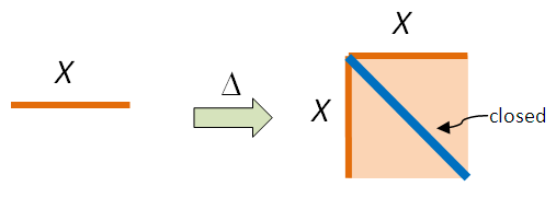
If X is Hausdorff, then any point outside the diagonal is of the form (x, y), x≠y. Pick disjoint open subsets U, V of X containing x, y respectively. Then $(x,y)\in U\times V\subseteq (X\times X) -\Delta(X).$ So (X×X)-Δ(X) is open.

Conversely, if W := (X×X)-Δ(X) is open, then for any distinct x, y in X, $(x,y)\in W$ must be contained in a basic open subset $(x,y)\in U\times V\subseteq W$ for some open $U, V\subseteq X.$ Then U, V are open subsets of X containing x, y respectively and they’re disjoint since U × V is a subset of W. ♦

It’s not hard to construct Hausdorff spaces from existing ones.

Theorem.

If $f:Y\to X$ is an injective continuous map and X is Hausdorff, then so is Y. In particular, a subspace of a Hausdorff space is Hausdorff.

If each $X_i$ is Hausdorff, then so is $X=\coprod_i X_i.$

If each $X_i$ is Hausdorff, then so is $X=\prod_i X_i.$

Proof

1st statement: if $a, b\in Y$ are disjoint, then so are f(a), f(b). Since X is Hausdorff, we can find disjoint open subsets U, V of X containing f(a), f(b) respectively. Then $f^{-1}(U), f^{-1}(V)$ are disjoint open subsets of Y containing a, b respectively.

2nd statement: given two distinct points of X, suppose they belong to distinct components $x\in X_i, y\in X_j, i\ne j.$ Then $X_i, X_j$ are the desired open subsets of X. Otherwise, $x,y\in X_i$ belong to the same component; since this is Hausdorff, we can find disjoint open subsets $U, V\subseteq X_i$ containing x, y respectively. But $X_i\subseteq X$ is open, hence so are $U, V\subseteq X.$

3rd statement: if $(x_i), (y_i)\in X$ are distinct, there’s an index i such that $x_i\ne y_i.$ Since $X_i$ is Hausdorff, we can find disjoint open subsets $U_i, V_i\subseteq X_i$ containing $x_i, y_i$ respectively. Then the open slices $(\prod_{j\ne i} X_j)\times U_i$ and $(\prod_{j\ne i}X_j)\times V_i$ are disjoint open subsets of X containing $(x_i), (y_i)$ respectively. ♦

Examples

As we noted earlier, any metric space is Hausdorff.
In particular, R, Rⁿ and any subspace of it are Hausdorff. Also, the discrete topological space is Hausdorff.
The coarsest topology on X, given by $T=\{\emptyset, X\}$ , is not Hausdorff if |X|>1.
N under the right order topology is not Hausdorff since any open subset containing 2 also contains 3. For the same reason, N* is also not Hausdorff.
An infinite set under the cofinite topology is not Hausdorff.

Dense Subsets

We define:

Definition. A subset Y of a topological space X is said to be dense if its closure cl(Y) = X.

Note that if $Y\subseteq Z\subseteq X,$ then saying Y is dense in Z means $\text{cl}_Z(Y) = Z.$ But since 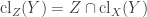$\text{cl}_Z(Y) = Z\cap \text{cl}_X(Y)$ this is equivalent to saying cl_X(Y) contains Z. In particular, given any subset Y of X, taking the closure in X gives $Y\subseteq \text{cl}_X(Y)\subseteq X.$ Setting Z = cl_X(Y), we see that Y is dense in Z.

The intuitive picture of a dense subset is one which almost fills up the entire space.

Here’s a useful characterisation of a dense subset.

Proposition. A subset Y of X is dense if and only if every non-empty open subset U of X intersects Y.

Proof.

We have Y is dense in X $\iff\text{cl}(Y) = X \iff \text{int}(X-Y) = \emptyset$ which holds if and only if X–Y has no non-empty subset open in X. This is the same as saying any non-empty open subset of X intersects Y. ♦

Examples

The open interval (0, 1) is dense in [0, 1].
The set of rationals Q is dense in R.
In N under the right order topology, any infinite subset is dense since it intersects any open subset {n, n+1, n+2, … }.
In N*, the singleton set {∞} is dense since it intersects any open subset.
In an infinite set X under the cofinite topology, any infinite subset is dense (since any closed subset is either the whole of X, or finite).

The following result explains in a more rigourous manner why Y “almost fills” X.

Proposition. Suppose $f, g : X\to Z$ are continuous functions to a Hausdorff space Z. If Y is a dense subset of X such that $f|_Y = g|_Y,$ then f=g.

Proof.

Suppose $f(x)\ne g(x)\in Z$ .

Pick disjoint open subsets U, V of Z containing f(x), g(x) respectively.
Now $x\in f^{-1}(U)\cap g^{-1}(V)=:W$ so W is a non-empty open subset of X.
Since Y is dense in X, we can find $y\in Y\cap W.$
Now since y lies in Y, f(y) = g(y). On the other hand, since y lies in W, $f(y)\in U$ and $g(y)\in V.$ Yet U, V are disjoint, which gives us a contradiction. ♦

Note

If Z is not Hausdorff, it’s easy to find counter-examples. E.g. let Z = {a, b} with the coarsest topology. Then any function R → Z is automatically continuous. In particular, two continuous functions can agree on R-{0} but disagree at 0.

We have the following properties for dense subsets (compare this with the case of Hausdorff spaces).

Proposition.

If $f : X \to Z$ is a surjective continuous map and Y is a dense subset of X, then f(Y) is dense in Z.

If each $Y_i\subseteq X_i$ is dense, then so is $\coprod_i Y_i \subseteq \coprod_i X_i.$

If each $Y_i\subseteq X_i$ is dense, then so is $\prod_i Y_i \subseteq \prod_i X_i.$

Proof.

1st statement: let V be a non-empty open subset of Z. Since f is surjective, f^-1(V) is a non-empty open subset of X. Since Y is dense in X, it must intersect f^-1(V). It follows that V must intersect f(Y).

2nd statement: let $U\subseteq \coprod_i X_i$ be open and non-empty. Then $U\cap X_i\ne \emptyset$ for some i. Since U ∩ X_i is a non-empty open subset of X_i, it must intersect Y_i, and hence, Y. Thus, U intersects Y.

3rd statement: follows from $\text{cl}(\prod_i Y_i) = \prod_i \text{cl}(Y_i).$ ♦

Note

Observe that the Hausdorff condition is preserved by injective maps while dense subsets are preserved by surjective maps. This makes sense intuitively since the Hausdorff condition separates points, and an injective map just separates them further. On the other hand, a dense subset attempts to fill up the space, so a surjective map packs it even more tightly.

Posted in Notes | Tagged advanced, continuity, dense subsets, Hausdorff, metric spaces, nets, topology | 4 Comments

Motivation

Separation Axioms

Combined Properties

Urysohn’s Lemma

Urysohn’s Metrisation Theorem

Locally Connected Spaces

Properties of Locally Connected Spaces

Locally Path-Connected Spaces

Non-Properties

Relationship Between (Locally) Connected & Path-connected

Summary

Path-Connected Components

Examples

Intermediate Value Theorem

Connected Components

Examples

Compactifications

One-Point Compactifications

Examples and Properties

Locally Compact Spaces

Properties of Locally Compact Spaces

Examples

Application: Infinite Four-Colour Theorem

Application: Infinite Tiling

Properties of Compact Spaces

Alexander’s Subbase Theorem

Zorn’s Lemma

Compact Spaces

Replacing Sequences with Nets

Completion of Metric Space

Exercise

Properties of the Completion

Existence of Completion

Hausdorff Spaces

Dense Subsets

Recent Posts

Archives

Categories

Meta

Pages