
Artinian Modules
Instead of the ascending chain condition, we can take its reverse.
Definition.
Let M be an A-module. Consider the set
of submodules of M, ordered by inclusion, i.e.
if and only if
. We say M is artinian if
The ring A is said to be artinian if it is artinian as a module over itself.
Again M is artinian if either of the following equivalent conditions holds.
- Every non-empty collection of submodules of M has a minimal element.
- If
is a sequence of submodules of M, then
for some
.
Examples
Let 
Let 


Exercise A
1. Prove that in an exact sequence of A-modules:

M is artinian if and only if N and P are. In particular, the direct sum of two artinian modules is artinian.
2. Prove that if M is a noetherian A-module, any surjective linear 
Decide if each of the following statements is true.
3. The product of any two artinian rings is artinian.
4. Any quotient of an artinian ring is artinian.
5. Any localization of an artinian ring is artinian.

Simple Modules
Let A be a fixed ring throughout this article and M be an A-module.
Definition.
M is said to be simple if it is non-zero and has no submodules except 0 and itself.
We immediately have the following.
Lemma 1.
M is simple if and only if
for some maximal ideal
.
Proof
(⇒) Pick a non-zero 


(⇐) Submodules of 

Example
Thus we see that simple modules over a coordinate ring k[V] (k algebraically closed) correspond to points on V. Even though we have 
Easy Exercise
Prove that for any ideals 


Composition Series
Next we would like to “factor” a module into its constituents comprising of simple modules.
Definition.
A composition series for M is a sequence of submodules
such that
is simple for all
. The length of the composition series is n; the composition factors of the series are the isomorphism classes of

Example
Let 


Recall that their scheme intersection (exercise D here) has coordinate ring
![\begin{aligned} A := k[W_1] \otimes_{k[V]} k[W_2] &\cong k[X, Y]/(Y - X^3 + 3X, Y - 2)\\ &\cong k[X]/(X^3 - 3X - 2)\\ &\cong k[X] / (X+1)^2 \times k[X] / (X-2) \end{aligned}](https://s0.wp.com/latex.php?latex=%5Cbegin%7Baligned%7D+A+%3A%3D+k%5BW_1%5D+%5Cotimes_%7Bk%5BV%5D%7D+k%5BW_2%5D+%26%5Ccong+k%5BX%2C+Y%5D%2F%28Y+-+X%5E3+%2B+3X%2C+Y+-+2%29%5C%5C+%26%5Ccong+k%5BX%5D%2F%28X%5E3+-+3X+-+2%29%5C%5C+%26%5Ccong+k%5BX%5D+%2F+%28X%2B1%29%5E2+%5Ctimes+k%5BX%5D+%2F+%28X-2%29+%5Cend%7Baligned%7D&bg=ffffff&fg=333333&s=0&c=20201002)
by Chinese Remainder Theorem. In fact, the above are all isomorphisms as algebras over ![k[V] = k[X, Y]](https://s0.wp.com/latex.php?latex=k%5BV%5D+%3D+k%5BX%2C+Y%5D&bg=ffffff&fg=333333&s=0&c=20201002)
![k[X]](https://s0.wp.com/latex.php?latex=k%5BX%5D&bg=ffffff&fg=333333&s=0&c=20201002)
![k[X, Y]/(Y)](https://s0.wp.com/latex.php?latex=k%5BX%2C+Y%5D%2F%28Y%29&bg=ffffff&fg=333333&s=0&c=20201002)

This has length 3; the composition factors are two copies of 

Proposition 1.
M has a composition series if and only if it is a noetherian and artinian module.
Proof
(⇒) Suppose 

(⇐) Conversely suppose M is both noetherian and artinian; we may assume 


Corollary 1.
If M has a composition series, so do any submodule and quotient module of M.
Uniqueness of Composition Series
Theorem 1.
Let M be a noetherian and artinian A-module. The composition factors of any composition series are unique up to isomorphism and reordering.
Note
For a composition series 

Proof
The proof is by contradiction; say a module is bad if it has two composition series with different sets of composition factors.
Step 1: Assume M is minimal.
Take the collection Σ of all bad submodules of M. Since M is artinian, we can replace M by a minimal element of Σ. Thus M has two composition series

such that 
Step 2: Consider the easy case.
Clearly 


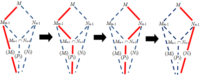
Step 3: Do the “diamond argument”.
Otherwise we have 

and similarly 
Step 4: Apply induction.
Pick any composition series 


The second and fourth equalities follow from the fact that 

This completes our proof. ♦
Corollary 2.
If M is a noetherian and artinian module, write
(length of M) for the length of any composition series of M. This is a well-defined value.
Similarly, we can define the composition factors of M and denote it by
.
Note that if 

This gives another application of short exact sequences.
Exercise B
1. Compute the length and composition series of
![B = \mathbb R[X]/ (X^6 + X^2)](https://s0.wp.com/latex.php?latex=B+%3D+%5Cmathbb+R%5BX%5D%2F+%28X%5E6+%2B+X%5E2%29&bg=ffffff&fg=333333&s=0&c=20201002)
as an B-module.
2. Prove that for a ring quotient 
In the next article, we will look at artinian rings. It turns out this is a small subclass of the collection of noetherian rings.
Optional Note
All the results in this section can be generalized to left modules over a non-commutative ring. This has applications in representation theory, since a simple module over the group algebra ![k[G]](https://s0.wp.com/latex.php?latex=k%5BG%5D&bg=ffffff&fg=333333&s=0&c=20201002)
 are non-empty open subsets then
  .
. are closed subsets whose union is X, then C = X or D = X.
 be non-empty open subsets. Then they are non-empty open subsets of X also, so
  . ♦
. ♦ be a non-empty dense subset of X. If Y is irreducible so is X.
 be the closure of A in X. We will use the topological fact: if
  then
then  .
. be a non-empty open subset. Since Y is dense in X,
  is a non-empty open subset of Y. We have
  , but since Y is irreducible
  . Hence
  . Since Y is dense in X we have
  . ♦
. ♦ be a continuous map. If X is irreducible, so is
  .
. be non-empty open subsets. Then
  are non-empty open subsets of X so
  . Thus
  . ♦
. ♦ .
. (
( open) form a basis of
  and
and  , where
  and
and  are open. Since these are all non-empty,
 . ♦
. ♦ . [ Warning: this is not the product topology, as we noted
  . Find a counter-example when k is not algebraically closed.
 is a sequence of closed subsets of X then for some n we have
  .
. It is possible for a non-noetherian ring to have a noetherian spectrum. For example if
 ![A = k[X_1, X_2, \ldots ]/(X_1^2, X_2^2, \ldots)](https://s0.wp.com/latex.php?latex=A+%3D+k%5BX_1%2C+X_2%2C+%5Cldots+%5D%2F%28X_1%5E2%2C+X_2%5E2%2C+%5Cldots%29&bg=ffffff&fg=333333&s=0&c=20201002) then A has exactly one prime ideal but it is not noetherian.
then A has exactly one prime ideal but it is not noetherian. are noetherian subspaces, then so is
  .
. .
. so
so  . It suffices to apply Zorn’s lemma to this set, so we need to show that any chain
  has an upper bound. Hence it suffices to show
  is irreducible.
 are disjoint non-empty open subsets. Then
  and
and  for some
  . Since
  is a chain we may assume without loss of generality that
  . This gives
  , non-empty disjoint open subsets of
  , which contradicts irreducibility of
  under (i) the usual topology, (ii) the cofinite topology (where the only closed subsets are the finite subsets and
  be irreducible components of X. If
  is irreducible then
  for some i.
 . In the latter case
  so by induction hypothesis
  for some
  . ♦
. ♦ . Furthermore, for any
  we have
 where
where  are closed subsets of C. Since
  is minimal we have
  . Thus each of them is a finite union of irreducible subsets, and so is C, a contradiction. ♦
 be the variety defined by the equations
 and hence
  or
or  . The first case gives the z-axis
  while the second case gives a hyperbola
  for
for  . Hence V has two irreducible components. The corresponding minimal primes of
 ![A = \mathbb C[X, Y, Z]/(X^2 - YZ, X^3 - Y)](https://s0.wp.com/latex.php?latex=A+%3D+%5Cmathbb+C%5BX%2C+Y%2C+Z%5D%2F%28X%5E2+-+YZ%2C+X%5E3+-+Y%29&bg=ffffff&fg=333333&s=0&c=20201002) are:
are:
 is exactly
  .
. with prime factorization
  , the radical of the principal ideal (b) is
  .
.![\mathbb C[X, Z]/(X^2 - X^3 Z)](https://s0.wp.com/latex.php?latex=%5Cmathbb+C%5BX%2C+Z%5D%2F%28X%5E2+-+X%5E3+Z%29&bg=ffffff&fg=333333&s=0&c=20201002) . Since
. Since ![\mathbb C[X, Z]](https://s0.wp.com/latex.php?latex=%5Cmathbb+C%5BX%2C+Z%5D&bg=ffffff&fg=333333&s=0&c=20201002) is a UFD, the radical of A is
is a UFD, the radical of A is  . Hence the intersection of all prime ideals of A is
  so
so
 . We say M is noetherian if
  is a sequence of submodules of M, then
  and
and  .
. be a sequence of submodules of M. We get sequences of submodules
 and
and  . Now apply the following to finish to job. ♦
 and N are submodules of M such that
  and
and  , then
  .
. .
. ).
). . If
. If  pick any
  . Then
  is a finitely generated submodule of M which properly contains
  of M. Let
  . Show that this is a submodule of M. By the given condition it is finitely generated by, say,
  . Then for some n we have
  . It follows that
  . ♦
. ♦ can be factored as a product of irreducibles.
 . And since
  is finitely generated, it is a quotient of some
  .
. .
. for some ideal
  . If
. If  is generated by
  then
then  is generated by
  . ♦
. ♦ .
. where
where  .
. where
where  is an ideal, so it is finitely generated. ♦
![A[X]](https://s0.wp.com/latex.php?latex=A%5BX%5D&bg=ffffff&fg=333333&s=0&c=20201002) .
.![\mathfrak b \subseteq A[X]](https://s0.wp.com/latex.php?latex=%5Cmathfrak+b+%5Csubseteq+A%5BX%5D&bg=ffffff&fg=333333&s=0&c=20201002) is not finitely generated; we pick
is not finitely generated; we pick  of minimum degree. Recursively, pick
  of minimum degree. Let
  so that
  . Suppose the leading term of
  is
is  , where
  .
. of ideals of A eventually terminates so
  for some n. We write
  for some
  . Now
. Now
 has degree
  and leading coefficient
  . Hence
  has degree
  and lies outside
  , which contradicts minimality of
  . ♦
. ♦![A[X_1, \ldots, X_n]](https://s0.wp.com/latex.php?latex=A%5BX_1%2C+%5Cldots%2C+X_n%5D&bg=ffffff&fg=333333&s=0&c=20201002) for some n. ♦
for some n. ♦ .
. is a fixed local ring.
 .
. , where
  is the
  is a minimal set of generators of M. If n = 0, M = 0 and we are done. Otherwise, we have
  so we can write
 , we have
  a unit, so in fact:
 (contradiction). ♦
 span it as a vector space over
  be the A-linear map which takes
  . Let C be the cokernel of f so we get an exact sequence of A-modules:
  . Since the functor
  is right-exact (by
 is surjective so
  . Since C is finitely generated (being a quotient of M), we have C = 0. ♦
 and pick
  such that
  form a basis over
  and
and  are minimal generating sets of M, then
 with entries in A.
 . More generally, for
  , the r-th order cotangent space of A is
  .
. .
. . The anomaly in exercise B thus does not occur. From Nakayama’s lemma, we see that a minimal generating set of
  over
over  , let
, let  so that
  . We can apply our above reasoning to the local ring
  and
and  . Note that
 .
.![A = k[X_1, \ldots, X_n]](https://s0.wp.com/latex.php?latex=A+%3D+k%5BX_1%2C+%5Cldots%2C+X_n%5D&bg=ffffff&fg=333333&s=0&c=20201002) and
and  . Then
  and
and  in non-negative integers. By elementary combinatorics, we have
![k[X_1, \ldots, X_n]](https://s0.wp.com/latex.php?latex=k%5BX_1%2C+%5Cldots%2C+X_n%5D&bg=ffffff&fg=333333&s=0&c=20201002) we will write
we will write  instead of
  for its image in A.
![A = k[X, Y]/(Y^2 - X^3 + X)](https://s0.wp.com/latex.php?latex=A+%3D+k%5BX%2C+Y%5D%2F%28Y%5E2+-+X%5E3+%2B+X%29&bg=ffffff&fg=333333&s=0&c=20201002) and
and  . Since
  in A, any monomial of degree r which contains
  lies in
  . Thus
  and
and
![A = k[X, Y, Z]/(Z^3 - X^3 - Y^3)](https://s0.wp.com/latex.php?latex=A+%3D+k%5BX%2C+Y%2C+Z%5D%2F%28Z%5E3+-+X%5E3+-+Y%5E3%29&bg=ffffff&fg=333333&s=0&c=20201002) and
and  . In
. In ![k[X, Y, Z]](https://s0.wp.com/latex.php?latex=k%5BX%2C+Y%2C+Z%5D&bg=ffffff&fg=333333&s=0&c=20201002) , the elements
, the elements  do not have any linear relation modulo
  , hence we have
  .
. so we have
  .
. where
where  , we have
  in A so a basis is given by
  where
where  and
and  . Thus
  . In conclusion
 can be represented by a polynomial for sufficiently large r. This is called the Hilbert polynomial of the local ring A; we shall have more to say about this later.
 which maps
 to obtain:
 ‘s form a minimal generating set of M over A,
  is an isomorphism and we have
  . By
. By  . ♦
. ♦

 be a surjective map where F is free; let K be its kernel so we get a short exact sequence
  . Since M and F are flat, we have a
  ,
,  is free over
  .
.
 and
and  for
for  . Then we get a long exact sequence:

 .
. so that
  .
. is surjective there exists
  ,
,  .
. .
. .
. for a unique
  .
. image of
  in
in  .
. in the second step, then
  . Thus
  for some
  so
so  and thus the new
  in the above construction is
  . So
. So  have the same image in
  .
. and
and  for A-modules M and N. Since any A-linear map
  induces a B-linear map
  we have a map
  . This is clearly A-linear so it induces a B-linear map
![[\mathrm{Hom}_A(M, N)]^B \longrightarrow \mathrm{Hom}_B(M^B, N^B), \quad b \otimes f \mapsto b\cdot f^B,](https://s0.wp.com/latex.php?latex=%5B%5Cmathrm%7BHom%7D_A%28M%2C+N%29%5D%5EB+%5Clongrightarrow+%5Cmathrm%7BHom%7D_B%28M%5EB%2C+N%5EB%29%2C+%5Cquad+b+%5Cotimes+f+%5Cmapsto+b%5Ccdot+f%5EB%2C&bg=ffffff&fg=333333&s=0&c=20201002)
 .
. where
where  are finite free modules. Since
  ,
,  making the diagram commute.
 .
. is finitely generated. Furthermore, since
  is finite free
  is finitely generated. Since
  and
and  are finitely generated so is K. ♦
 , if N and P are finitely presented, so is M.
 if there is an exact sequence
 is finite free.
 means it is finitely generated and saying M is
  means it is finitely presented. One can show more generally that if M has type
  has type
  . However, this is outside our scope of discussion.
![[\mathrm{Hom}_A(M, N)]^B \stackrel \cong \longrightarrow \mathrm{Hom}_B(M^B, N^B), \quad b \otimes f \mapsto b\cdot f^B.](https://s0.wp.com/latex.php?latex=%5B%5Cmathrm%7BHom%7D_A%28M%2C+N%29%5D%5EB+%5Cstackrel+%5Ccong+%5Clongrightarrow+%5Cmathrm%7BHom%7D_B%28M%5EB%2C+N%5EB%29%2C+%5Cquad+b+%5Cotimes+f+%5Cmapsto+b%5Ccdot+f%5EB.&bg=ffffff&fg=333333&s=0&c=20201002)
 . Since
 is exact, we get an exact sequence of B-modules
![0 \longrightarrow [\mathrm{Hom}_A (M, N)]^B \stackrel {(g^*)^B} \longrightarrow [\mathrm{Hom}_A(A^n, N)]^B \stackrel {(f^*)^B } \longrightarrow [\mathrm{Hom}_A(A^m, N)]^B.](https://s0.wp.com/latex.php?latex=0+%5Clongrightarrow+%5B%5Cmathrm%7BHom%7D_A+%28M%2C+N%29%5D%5EB+%5Cstackrel+%7B%28g%5E%2A%29%5EB%7D+%5Clongrightarrow+%5B%5Cmathrm%7BHom%7D_A%28A%5En%2C+N%29%5D%5EB+%5Cstackrel+%7B%28f%5E%2A%29%5EB+%7D+%5Clongrightarrow+%5B%5Cmathrm%7BHom%7D_A%28A%5Em%2C+N%29%5D%5EB.&bg=ffffff&fg=333333&s=0&c=20201002)


![[\mathrm{Hom}_A(A^n, N)]^B \cong (N^n)^B \cong (N^B)^n \cong \mathrm{Hom}_B(B^n, N^B)](https://s0.wp.com/latex.php?latex=%5B%5Cmathrm%7BHom%7D_A%28A%5En%2C+N%29%5D%5EB+%5Ccong+%28N%5En%29%5EB+%5Ccong+%28N%5EB%29%5En+%5Ccong+%5Cmathrm%7BHom%7D_B%28B%5En%2C+N%5EB%29&bg=ffffff&fg=333333&s=0&c=20201002)
![[\mathrm{Hom}_A(M, N)]^B \longrightarrow \mathrm{Hom}_B(M^B, N^B)](https://s0.wp.com/latex.php?latex=%5B%5Cmathrm%7BHom%7D_A%28M%2C+N%29%5D%5EB+%5Clongrightarrow+%5Cmathrm%7BHom%7D_B%28M%5EB%2C+N%5EB%29&bg=ffffff&fg=333333&s=0&c=20201002) . Hence this map is an isomorphism. ♦
. Hence this map is an isomorphism. ♦ , as a special case we obtain the following.
 .
. be a surjective
 , we get a surjective:
 be a surjective A-linear map. We need to show
 is surjective for all maximal
 , we call it an
  –torsion element.
 (where
  . Hence M has no a-torsion elements other than 0. ♦
![A = k[X] \longrightarrow k[X, Y, Z]/(XZ, YZ) = B.](https://s0.wp.com/latex.php?latex=A+%3D+k%5BX%5D+%5Clongrightarrow+k%5BX%2C+Y%2C+Z%5D%2F%28XZ%2C+YZ%29+%3D+B.&bg=ffffff&fg=333333&s=0&c=20201002)
 so it is not A-flat. The homomorphism corresponds to a morphism f from the variety
  to
to  by projecting onto the x-coordinate. We treat W as a collection of varieties parametrized by points on V, with
  .
.
 , we have
  . And when
  , we have
  , a union of two lines. On an intuitive level, this means
  , although such a statement makes no sense here.
![k[V] \to k[W]](https://s0.wp.com/latex.php?latex=k%5BV%5D+%5Cto+k%5BW%5D&bg=ffffff&fg=333333&s=0&c=20201002) is flat, then
is flat, then  gives a family of varieties “smoothly parametrized” by elements of V.
 ; we get the restriction
  where
where  . Taking the Zariski closure in their respective spaces gives us
![k[W^\circ] \cong k[X, Y]](https://s0.wp.com/latex.php?latex=k%5BW%5E%5Ccirc%5D+%5Ccong+k%5BX%2C+Y%5D&bg=ffffff&fg=333333&s=0&c=20201002) and the homomorphism of coordinate rings is
and the homomorphism of coordinate rings is ![k[X]\hookrightarrow k[X, Y]](https://s0.wp.com/latex.php?latex=k%5BX%5D%5Chookrightarrow+k%5BX%2C+Y%5D&bg=ffffff&fg=333333&s=0&c=20201002) . This extension is flat since it is free.
. This extension is flat since it is free. is not dense in W even though U is dense in V.
 be a morphism of k-varieties with corresponding
![f^* : A := k[V] \longrightarrow k[W] =: B.](https://s0.wp.com/latex.php?latex=f%5E%2A+%3A+A+%3A%3D+k%5BV%5D+%5Clongrightarrow+k%5BW%5D+%3D%3A+B.&bg=ffffff&fg=333333&s=0&c=20201002)
 for
for ![g\in k[V]](https://s0.wp.com/latex.php?latex=g%5Cin+k%5BV%5D&bg=ffffff&fg=333333&s=0&c=20201002) ; recall
; recall  .
. is dense in V if and only if g is not a zero-divisor.
 is exactly
  .
.![k[V][\frac 1 g]](https://s0.wp.com/latex.php?latex=k%5BV%5D%5B%5Cfrac+1+g%5D&bg=ffffff&fg=333333&s=0&c=20201002) and
and ![k[W][\frac 1 g]](https://s0.wp.com/latex.php?latex=k%5BW%5D%5B%5Cfrac+1+g%5D&bg=ffffff&fg=333333&s=0&c=20201002) respectively. The geometric condition “if
respectively. The geometric condition “if ![k[W]](https://s0.wp.com/latex.php?latex=k%5BW%5D&bg=ffffff&fg=333333&s=0&c=20201002) has no g-torsion”.
has no g-torsion”.![A \subset A[X] \subset A[X, \frac 1 X]](https://s0.wp.com/latex.php?latex=A+%5Csubset+A%5BX%5D+%5Csubset+A%5BX%2C+%5Cfrac+1+X%5D&bg=ffffff&fg=333333&s=0&c=20201002) . The first inclusion is flat because
. The first inclusion is flat because ![A[X, \frac 1 X]](https://s0.wp.com/latex.php?latex=A%5BX%2C+%5Cfrac+1+X%5D&bg=ffffff&fg=333333&s=0&c=20201002) is a flat A-algebra.
is a flat A-algebra.![k[X] \subset k[X, Y]/(XY)](https://s0.wp.com/latex.php?latex=k%5BX%5D+%5Csubset+k%5BX%2C+Y%5D%2F%28XY%29&bg=ffffff&fg=333333&s=0&c=20201002) is not flat because X becomes a zero-divisor in
is not flat because X becomes a zero-divisor in ![k[X, Y]/(XY)](https://s0.wp.com/latex.php?latex=k%5BX%2C+Y%5D%2F%28XY%29&bg=ffffff&fg=333333&s=0&c=20201002) .
.![k[X, Y]/(XY) \to k[X]](https://s0.wp.com/latex.php?latex=k%5BX%2C+Y%5D%2F%28XY%29+%5Cto+k%5BX%5D&bg=ffffff&fg=333333&s=0&c=20201002) taking
taking  ? This is also not A-flat. For that we note that
  .
. . Taking
  gives us, together with
  , we get the exact sequence
 . ♦
. ♦ since
since  .
. of a ring A which satisfies
  and
and  with
with  , which corresponds to
![A = k[X, Y]/(Y^2 - X^3) \longrightarrow k[T] = B, \quad X \mapsto T^2, Y \mapsto T^3.](https://s0.wp.com/latex.php?latex=A+%3D+k%5BX%2C+Y%5D%2F%28Y%5E2+-+X%5E3%29+%5Clongrightarrow+k%5BT%5D+%3D+B%2C+%5Cquad+X+%5Cmapsto+T%5E2%2C+Y+%5Cmapsto+T%5E3.&bg=ffffff&fg=333333&s=0&c=20201002)
 be a maximal ideal. It suffices to show that the product map
  not injective. Indeed
  both map to
  . On the other hand, they are distinct elements of
  . To see why we take
 factors through
  and
and  ; in particular
  in
in  .
. is flat, then so is
  . But
. But  so the resulting map is
![k[X, Y]/(Y^2 - X^3, X) \cong k[Y]/(Y^2) \longrightarrow k[T]/(T^2), \quad Y \mapsto 0](https://s0.wp.com/latex.php?latex=k%5BX%2C+Y%5D%2F%28Y%5E2+-+X%5E3%2C+X%29+%5Ccong+k%5BY%5D%2F%28Y%5E2%29+%5Clongrightarrow+k%5BT%5D%2F%28T%5E2%29%2C+%5Cquad+Y+%5Cmapsto+0&bg=ffffff&fg=333333&s=0&c=20201002) .
.![k[Y]/(Y^2) \to k \hookrightarrow k[T]/(T^2)](https://s0.wp.com/latex.php?latex=k%5BY%5D%2F%28Y%5E2%29+%5Cto+k+%5Chookrightarrow+k%5BT%5D%2F%28T%5E2%29&bg=ffffff&fg=333333&s=0&c=20201002) . The first map is not flat by applying lemma 2 to the ideal
. The first map is not flat by applying lemma 2 to the ideal  of ring
 ![A' = k[Y]/(Y^2)](https://s0.wp.com/latex.php?latex=A%27+%3D+k%5BY%5D%2F%28Y%5E2%29&bg=ffffff&fg=333333&s=0&c=20201002) . Specifically the injective map
. Specifically the injective map  , upon applying the functor
  , gives us
  taking
 ![k[T]/(T^2)](https://s0.wp.com/latex.php?latex=k%5BT%5D%2F%28T%5E2%29&bg=ffffff&fg=333333&s=0&c=20201002) is free over k, upon applying
is free over k, upon applying ![k[T]/(T^2) \otimes_k -](https://s0.wp.com/latex.php?latex=k%5BT%5D%2F%28T%5E2%29+%5Cotimes_k+-&bg=ffffff&fg=333333&s=0&c=20201002) , the map is still not injective.
, the map is still not injective. parametrized by a, b, c from
 ![f : k[A, B, C] \hookrightarrow k[A, B, C, X, Y]/(AX^2 + BY^2 - C)](https://s0.wp.com/latex.php?latex=f+%3A+k%5BA%2C+B%2C+C%5D+%5Chookrightarrow+k%5BA%2C+B%2C+C%2C+X%2C+Y%5D%2F%28AX%5E2+%2B+BY%5E2+-+C%29&bg=ffffff&fg=333333&s=0&c=20201002) .
.![f' : k[A] \hookrightarrow k[A, X, Y]/(AX^2)](https://s0.wp.com/latex.php?latex=f%27+%3A+k%5BA%5D+%5Chookrightarrow+k%5BA%2C+X%2C+Y%5D%2F%28AX%5E2%29&bg=ffffff&fg=333333&s=0&c=20201002)
 is an A-torsion element, so we are done.
![k[T] \hookrightarrow k[X, Y, T]/(Y - TX^2)](https://s0.wp.com/latex.php?latex=k%5BT%5D+%5Chookrightarrow+k%5BX%2C+Y%2C+T%5D%2F%28Y+-+TX%5E2%29&bg=ffffff&fg=333333&s=0&c=20201002) a flat extension? What if we restrict to
a flat extension? What if we restrict to  ?
?![k[T] \hookrightarrow k[X,Y,T]/(XY - T)](https://s0.wp.com/latex.php?latex=k%5BT%5D+%5Chookrightarrow+k%5BX%2CY%2CT%5D%2F%28XY+-+T%29&bg=ffffff&fg=333333&s=0&c=20201002) .
. , i.e. we get the extension
![k[A, B, C, \frac 1 B] \hookrightarrow k[A, B, C, \frac 1 B, X, Y]/(AX^2 + BY^2 - C)](https://s0.wp.com/latex.php?latex=k%5BA%2C+B%2C+C%2C+%5Cfrac+1+B%5D+%5Chookrightarrow+k%5BA%2C+B%2C+C%2C+%5Cfrac+1+B%2C+X%2C+Y%5D%2F%28AX%5E2+%2B+BY%5E2+-+C%29&bg=ffffff&fg=333333&s=0&c=20201002) .
. , the family of ellipses
  is well-behaved. What about the open subset
  ?
? is a right-exact functor.
 is an exact functor, equivalently, if
 is flat if the resulting A-algebra structure on B is flat.
 is a collection of A-flat modules, then
  is A-flat.
 ♦
♦ . Then use the fact that localization functors are exact (
 is also flat.
 is free for some A-module Q. Thus
  ♦
♦ .
. is B-flat for any B-algebra.
 and ideal
  maintain some consistency over various
  . We will see some concrete examples in the next article.
 is an
is an  as
as  be an injective map of
 is injective, and hence so is
  .
. be an injective homomorphism of A-modules. From
  is injective if and only if
  is injective for each
 . Since
  is injective, we are done. ♦
 and
and  , the localization
  is
is  -flat.
 is invertible in
  is flat over
  is a further localization of
  and
and  . Let
. Let  be an injective map of A-modules and let K be the kernel of
  so we have an exact sequence of B-modules

 (exercise). And since
  for all maximal
  and
and  . ♦
. ♦ by multiplication.
 ,
, . ♦
. ♦ for all finitely generated ideals
 , then
  .
. .
. , we have
  .
. . And since
  is exact, we can apply many of the
  .
. is an A-linear map of ideals, we obtain an induced A-linear
  ,
,  .
. ; then
  .
. of ideals of A and an A-module M, such that the A-linear map
  ,
,  is not well-defined. Thus property 6 is non-trivial.
 ?
? has a natural structure of an A-algebra which satisfies
 .
. . The map
  is A-bilinear so it induces an A-linear map
 ,
,  so it induces an A-linear
 . Note that A-bilinearity means distributivity in either term. To prove associativity, show that it holds on the pure tensors (exercise). ♦
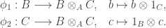
 ,
,  are A-algebra homomorphisms, then there is a unique A-algebra homomorphism
  such that
  and
and  .
. induces the A-linear map
 .
. .
. for
for  , and conversely, any such f must satisfy
  which uniquely determines f. ♦

 is an object, and
  is the
  in
in  we have a natural isomorphism
 is the canonical map and
  is the
 ![B \otimes_A A[X] \cong B[X]](https://s0.wp.com/latex.php?latex=B+%5Cotimes_A+A%5BX%5D+%5Ccong+B%5BX%5D&bg=ffffff&fg=333333&s=0&c=20201002) for any A-algebra B. There is more than one way to show it.
for any A-algebra B. There is more than one way to show it. for
for  , so
, so ![B \otimes_A A[X]](https://s0.wp.com/latex.php?latex=B+%5Cotimes_A+A%5BX%5D&bg=ffffff&fg=333333&s=0&c=20201002) is free over B with the same basis. Show that product in this ring still satisfies
is free over B with the same basis. Show that product in this ring still satisfies  so it is isomorphic to
 ![B[X]](https://s0.wp.com/latex.php?latex=B%5BX%5D&bg=ffffff&fg=333333&s=0&c=20201002) .
.![\mathrm{Hom}_{B\text{-alg}}(B \otimes_A A[X], C) \cong \mathrm{Hom}_{A\text{-alg}}(A[X], C) \cong C](https://s0.wp.com/latex.php?latex=%5Cmathrm%7BHom%7D_%7BB%5Ctext%7B-alg%7D%7D%28B+%5Cotimes_A+A%5BX%5D%2C+C%29+%5Ccong+%5Cmathrm%7BHom%7D_%7BA%5Ctext%7B-alg%7D%7D%28A%5BX%5D%2C+C%29+%5Ccong+C&bg=ffffff&fg=333333&s=0&c=20201002)
![\mathrm{Hom}_{B\text{-alg}} (B[X], C)\cong C](https://s0.wp.com/latex.php?latex=%5Cmathrm%7BHom%7D_%7BB%5Ctext%7B-alg%7D%7D+%28B%5BX%5D%2C+C%29%5Ccong+C&bg=ffffff&fg=333333&s=0&c=20201002) , the result follows by
, the result follows by  as A-modules as we saw earlier. Clearly the isomorphism preserves the ring structure so we get an isomorphism of A-modules.
 where
where  .
. ? This is the set of primes
  such that
 under the continuous map
  .
. as A-modules. Again it is in fact an isomorphism of A-algebras. Now
  is the set of primes
  such that
 .
. .
. .
.![B =A[X_1, \ldots X_n]/(f_i)](https://s0.wp.com/latex.php?latex=B+%3DA%5BX_1%2C+%5Cldots+X_n%5D%2F%28f_i%29&bg=ffffff&fg=333333&s=0&c=20201002) where
where ![f_i\in A[X_1, \ldots, X_n]](https://s0.wp.com/latex.php?latex=f_i%5Cin+A%5BX_1%2C+%5Cldots%2C+X_n%5D&bg=ffffff&fg=333333&s=0&c=20201002) is a collection of polynomials. Describe the functor
is a collection of polynomials. Describe the functor  be a prime ideal. Substitute
  in example 4 and
  in example 3. Thus the set of
  such that
 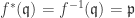 is given by:
 is the
  be a morphism of affine k-schemes, which corresponds to a ring homomorphism
 ![f :k[W] \to k[V]](https://s0.wp.com/latex.php?latex=f+%3Ak%5BW%5D+%5Cto+k%5BV%5D&bg=ffffff&fg=333333&s=0&c=20201002) . For a given point
. For a given point  , its fibre is the affine k-scheme
  with coordinate ring:
![k[\phi^{-1}(P)] = (k[W]/\mathfrak m_P) \otimes_{k[W]} k[V] \cong k[V]/f(\mathfrak m_P) k[V].](https://s0.wp.com/latex.php?latex=k%5B%5Cphi%5E%7B-1%7D%28P%29%5D+%3D+%28k%5BW%5D%2F%5Cmathfrak+m_P%29+%5Cotimes_%7Bk%5BW%5D%7D+k%5BV%5D+%5Ccong+k%5BV%5D%2Ff%28%5Cmathfrak+m_P%29+k%5BV%5D.&bg=ffffff&fg=333333&s=0&c=20201002)
 and
and  with morphism
  ,
,  . Algebraically, this is:
 , we have
  so that
![\begin{aligned} k[\phi^{-1}(P)] &= k[A, B, C, X, Y]/(AX^2 + BY^2 - C, A-1, B-1, C-1)\\ &\cong k[X, Y]/(X^2 + Y^2 - 1).\end{aligned}](https://s0.wp.com/latex.php?latex=%5Cbegin%7Baligned%7D+k%5B%5Cphi%5E%7B-1%7D%28P%29%5D+%26%3D+k%5BA%2C+B%2C+C%2C+X%2C+Y%5D%2F%28AX%5E2+%2B+BY%5E2+-+C%2C+A-1%2C+B-1%2C+C-1%29%5C%5C+%26%5Ccong+k%5BX%2C+Y%5D%2F%28X%5E2+%2B+Y%5E2+-+1%29.%5Cend%7Baligned%7D&bg=ffffff&fg=333333&s=0&c=20201002)
 , on the other hand, gives
 ![k[\phi^{-1}(Q)] \cong k[X, Y]](https://s0.wp.com/latex.php?latex=k%5B%5Cphi%5E%7B-1%7D%28Q%29%5D+%5Ccong+k%5BX%2C+Y%5D&bg=ffffff&fg=333333&s=0&c=20201002) .
. ,
,  are closed subsets. Then
  is also closed, being cut out by the same equations which define V and W, but with disjoint sets of variables.
 as an easy exercise.
![k[V\times W] \cong k[V] \otimes_k k[W]](https://s0.wp.com/latex.php?latex=k%5BV%5Ctimes+W%5D+%5Ccong+k%5BV%5D+%5Cotimes_k+k%5BW%5D&bg=ffffff&fg=333333&s=0&c=20201002) .
. induce k-algebra homomorphisms
 ![k[V], k[W] \to k[V\times W]](https://s0.wp.com/latex.php?latex=k%5BV%5D%2C+k%5BW%5D+%5Cto+k%5BV%5Ctimes+W%5D&bg=ffffff&fg=333333&s=0&c=20201002) and hence
and hence ![h : k[V]\otimes_k k[W] \to k[V\times W]](https://s0.wp.com/latex.php?latex=h+%3A+k%5BV%5D%5Cotimes_k+k%5BW%5D+%5Cto+k%5BV%5Ctimes+W%5D&bg=ffffff&fg=333333&s=0&c=20201002) ; h is surjective by our concrete description of
; h is surjective by our concrete description of ![k[V]](https://s0.wp.com/latex.php?latex=k%5BV%5D&bg=ffffff&fg=333333&s=0&c=20201002) . Suppose
. Suppose  for some
  and
and ![g_1, \ldots, g_n \in k[W]](https://s0.wp.com/latex.php?latex=g_1%2C+%5Cldots%2C+g_n+%5Cin+k%5BW%5D&bg=ffffff&fg=333333&s=0&c=20201002) . Thus
. Thus .
. which holds in
  for all
  so each
  and
and  . ♦
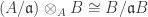
. ♦ be closed subvarieties of a variety V. This induces surjective k-algebra homomorphisms
 ![k[V] \to k[W_1]](https://s0.wp.com/latex.php?latex=k%5BV%5D+%5Cto+k%5BW_1%5D&bg=ffffff&fg=333333&s=0&c=20201002) and
and ![k[V] \to k[W_2]](https://s0.wp.com/latex.php?latex=k%5BV%5D+%5Cto+k%5BW_2%5D&bg=ffffff&fg=333333&s=0&c=20201002) . Write down the coordinate ring of the scheme intersection
. Write down the coordinate ring of the scheme intersection  using the language of tensor product.
 , we have:
 which takes
  . Note that this is well-defined: since only finitely many
  are non-zero, only finitely many
  are non-zero. It is A-bilinear so we have an induced A-linear map
 (resp.
  . Write
  and
and  . Distributivity together with
  gives us:
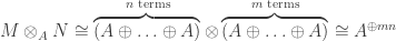
 over
over  . More generally:
 , i.e. a tensor product of free modules is free.
 where
where  corresponds to
  . Clearly B corresponds to a linear map
  , via
, via  . Hence we get the desired bijection. It is easy to show that the map is A-linear. ♦
 is functorial.
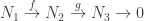 be an exact sequence.
 is exact, by

 and once for
  . ♦
. ♦ .
. be defined by
  . Then
  is the induced module.
 , there is a unique B-linear
  such that
  .
. which takes
  . This is clearly A-bilinear so it induces an A-linear
  which takes
  . It follows that
  .
. ; since f is B-linear,
  . Since every element of
  is a finite sum of
  we see that f must be as defined above. ♦
 is a generalization of these cases we have already seen.
 , by
, by  . Show that this is well-defined (i.e. independent of choice of a and s). So we get an A-linear map
  as above.
 via
via  . To show this is well-defined, if
  then
then  for some
  which gives
 .
. be an ideal.
 .
. is right-exact.
 which takes
  . Also define the reverse map
  by
by  . ♦
. ♦![B = A[X]](https://s0.wp.com/latex.php?latex=B+%3D+A%5BX%5D&bg=ffffff&fg=333333&s=0&c=20201002) and an A-module M, describe the induced A[X]-module
and an A-module M, describe the induced A[X]-module 
 is A-linear, let
  and
and  be the maps in the universal property. We leave it to the reader to fill out the remainder of the proof to obtain a B-linear

 as C-modules. ♦
 .
. we have


 . Multiplying both sides by
  gives:
 is a finite sum of
  , the result follows. ♦
 and
and  are real vector spaces, then
  is the vector space with basis
  over
over  . Hence it follows that
  .
. is the complex vector space of all
  where
where  . Thus
  .
.
 is A-linear;
 , the function
  is A-linear.
 and a linear
  for all
  .
.
 is a module,
 is bilinear, there is a unique linear map
  such that
  .
. with a, b real. Now take the bilinear
 .
. be the free A-module generated by
  for
for  . Now let P be the quotient of F by the submodule generated by elements of the form:
 . The map
  is defined by
  ; by definition of P this is A-bilinear.
 forms the tensor product of M and N.
 be any bilinear map. We first define a linear
  by taking
  . This map factors through P because:
 and thus
  takes
takes  to 0; Similarly it also takes all elements of the form
  ,
,  and
and  to zero.
 which takes
  . We have
 . But the set of
  generates F so this proves uniqueness. ♦
 , any
, any  , denoted by
  . The universal property of tensor product thus says the following.
 which sends
  .
. ; but in general not every element is of the form
  and
and  are linear maps, they induce a linear
  satisfying
  . We denote this map by
  .
.
 is not injective in general. Thus the functor
  does not take injective maps to injective maps. An example will be given at the end of this article.
 , where
  .
.
 ,
,  . This is easily checked to be A-bilinear so it induces an
  satisfying
  .
. , which is A-linear. It remains to show the maps are mutually inverse. Let
  due to bilinearity. Since the pure tensors
  generate
  we have
  .
. so
so  too. ♦
 which takes
  . This is an A-bilinear map so it induces a linear
 which takes
  is A-bilinear so it induces a linear
 which takes
  . Thus
  takes elements of the form
  back to themselves; since these generate the whole module we have
 , the multiplication-by-2 map. Taking
  gives us
  , still multiplication-by-2 but now it is the zero map. Hence tensor products do not take injective maps to injective maps in general.