Nakayama’s Lemma

The following is a short statement which has far-reaching applications. Since its main applications are for local rings, we will state the result in this context. Throughout this section, $(A, \mathfrak m)$ is a fixed local ring.

Theorem (Nakayama’s Lemma).

Let M be a finitely generated A-module. Then

$\mathfrak m M = M \implies M = 0$ .

In other words, if $M\ne 0$ then $k(\mathfrak m) \otimes M \cong M/\mathfrak m M \ne 0$ , where $k(\mathfrak m)$ is the residue field.

Proof (Lang)

Suppose $m_1, \ldots, m_n \in M$ is a minimal set of generators of M. If n = 0, M = 0 and we are done. Otherwise, we have $m_1 \in M = \mathfrak m M$ so we can write

$m_1 = a_1 m_1 + \ldots + a_n m_n, \quad a_1, \ldots, a_n \in \mathfrak m.$

But since $a_1 \in \mathfrak m$ , we have $1-a_1 \in A$ a unit, so in fact:

$m_1 = (1 - a_1)^{-1} (a_2 m_2 + \ldots + a_n m_n)$

and M has a smaller set of generators given by $m_2, \ldots, m_n$ (contradiction). ♦

Corollary 1.

Let M be a finitely generated module over $(A, \mathfrak m)$ and $m_1, \ldots, m_n \in M$ . If $\overline m_1, \ldots, \overline m_n \in M/\mathfrak m M$ span it as a vector space over $A/\mathfrak m$ , then $m_1, \ldots, m_n \in M$ generate it as an A-module.

Proof

Let $f:A^n \to M$ be the A-linear map which takes $e_i \mapsto m_i$ . Let C be the cokernel of f so we get an exact sequence of A-modules: $A^n \stackrel f \to M \to C \to 0$ . Since the functor $N \mapsto N/\mathfrak m N$ is right-exact (by corollary 2 here), we get an exact:

$(A/\mathfrak m)^n \stackrel{\overline f}\longrightarrow M/\mathfrak m M \longrightarrow C/\mathfrak m C \longrightarrow 0$

By the given condition $\overline f$ is surjective so $C = \mathfrak m C$ . Since C is finitely generated (being a quotient of M), we have C = 0. ♦

Hence, for a finitely generated M over $(A, \mathfrak m)$ , let $n = \dim_{A/\mathfrak m} M/\mathfrak m M$ and pick $m_1, \ldots, m_n$ such that $\overline m_i \in M/\mathfrak m M$ form a basis over $A/\mathfrak m$ . Then $m_1, \ldots, m_n$ form a minimal generating set for M over A. Furthermore, all minimal generating sets of M have the same cardinality: n.

Exercise A

Prove that if $\{m_1, \ldots, m_n\}$ and $\{m_1', \ldots, m_n'\}$ are minimal generating sets of M, then

$\begin{pmatrix} a_{11} & a_{12} & \ldots & a_{1n} \\ a_{21} & a_{22} & \ldots & a_{2n} \\ \vdots & \vdots & \ddots & \vdots \\ a_{n1} & a_{n2} & \ldots & a_{nn} \end{pmatrix} \begin{pmatrix} m_1 \\ m_2 \\ \vdots \\ m_n\end{pmatrix} = \begin{pmatrix} m_1 \\ m_2 \\ \vdots \\m_n\end{pmatrix}$

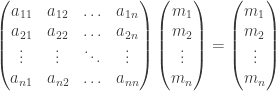
for some invertible matrix $(a_{ij})$ with entries in A.

blue-lin

Cotangent Spaces

Again $(A, \mathfrak m)$ denotes a local ring. Inspired by our earlier computation of tangent spaces, we define:

Definition.

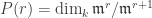
The cotangent space of A is given by $\mathfrak m / \mathfrak m^2$ . More generally, for $r\ge 1$ , the r-th order cotangent space of A is $\mathfrak m^r / \mathfrak m^{r+1}$ .

Exercise B

Find a local ring $(A, \mathfrak m)$ which is not a field, satisfying $\mathfrak m = \mathfrak m^2$ .

[ Hint: take the ring of all differentiable functions ℝ → ℝ and consider the maximal ideal of all functions vanishing at 0. ]

Let us assume that $\mathfrak m$ is a finitely generated module; hence so is every $\mathfrak m^r$ . The anomaly in exercise B thus does not occur. From Nakayama’s lemma, we see that a minimal generating set of $\mathfrak m^r$ is obtained from a basis of $\mathfrak m^r/ \mathfrak m^{r+1}$ over $A/\mathfrak m$ .

In the following examples, we will let A be the coordinate ring of a variety V over k (algebraically closed field). For $P\in V$ , let $\mathfrak m = \mathfrak m_P$ so that $A/\mathfrak m \cong k$ . We can apply our above reasoning to the local ring $B := A_{\mathfrak m}$ and $\mathfrak n = \mathfrak m B$ . Note that

$\mathfrak n^r /\mathfrak n^{r+1} \cong \mathfrak m^r / \mathfrak m^{r+1}$

since the RHS is already a B-module. Thus we only need to compute:

$P(r) = \dim_{k} \mathfrak m^r / \mathfrak m^{r+1}$

to find the minimum number of generators of $\mathfrak n^r$ .

Example 1

Suppose $A = k[X_1, \ldots, X_n]$ and $\mathfrak m = (X_1, \ldots, X_n)$ . Then $A / \mathfrak m = k$ and $\mathfrak m^r / \mathfrak m^{r+1}$ has k-basis given by all monomials of degree r. The number of such monomials is the number of solutions to $a_1 + \ldots + a_n = r$ in non-negative integers. By elementary combinatorics, we have

$P(r) = {r+n-1 \choose n-1},$

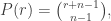
which is polynomial in r of degree n-1.

In the following examples, when A is a quotient of $k[X_1, \ldots, X_n]$ we will write $X_i$ instead of $\overline X_i$ for its image in A.

Example 2

Let $A = k[X, Y]/(Y^2 - X^3 + X)$ and $\mathfrak m =(X, Y)$ . Since $X = X^3 - Y^2 \in \mathfrak m^2$ in A, any monomial of degree r which contains $X$ lies in $\mathfrak m^{r+1}$ . Thus $\mathfrak m^r / \mathfrak m^{r+1}$ has basis $Y^r$ and

$P(r) = \dim_k (\mathfrak m^r / \mathfrak m^{r+1}) = 1.$

Example 3

Let $A = k[X, Y, Z]/(Z^3 - X^3 - Y^3)$ and $\mathfrak m = (X, Y, Z)$ . In $k[X, Y, Z]$ , the elements $X, Y, Z$ do not have any linear relation modulo $(X, Y, Z)^2 + (Z^3 - X^3 - Y^3) = (X, Y, Z)^2$ , hence we have $\dim_k \mathfrak m/\mathfrak m^2 = 3$ .

Similarly, in $k[X, Y, Z]$ the monomials of degree 2 have no linear relation modulo $(X, Y, Z)^3 + (Z^3 - X^3 - Y^3) = (X, Y, Z)^3$ so we have $\dim_k \mathfrak m^2 / \mathfrak m^3 = 6$ .

For $\mathfrak m^r /\mathfrak m^{r+1}$ where $r\ge 3$ , we have $Z^3 = X^3 + Y^3$ in A so a basis is given by $X^a Y^b Z^c$ where $a+b+c = r$ and $c=0,1,2$ . Thus $P(r) = 3r$ . In conclusion

$P(r) = \begin{cases} 1, \quad &\text{if } r = 0,\\ 3r, &\text{if } r\ge 1.\end{cases}$

Note

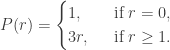
We thus see that in all three case, the function $P(r)$ can be represented by a polynomial for sufficiently large r. This is called the Hilbert polynomial of the local ring A; we shall have more to say about this later.

Question to Ponder

What can we say about the degree of the Hilbert polynomial?

blue-lin

F. P. + Flat = F. G. + Projective

Finally, here is an interesting result. Recall that saying a module is finite presented is a stronger condition than saying it is finitely generated. On the other hand, by corollary 1 here, projective modules are flat. It turns out these two pairs of properties complement each other.

Proposition 1.

An A-module M is finitely presented and flat if and only if it is finitely generated and projective.

Note

Let us keep stock of what we already know; by the above remarks f.p. ⇒ f.g. and flat ⇐ projective. By exercise A.2 here, f.p. ⇐ f.g. + projective. Thus the only remaining case is f.p. + flat ⇒ projective.

Proof

By localization, we may assume $(A, \mathfrak m)$ is local (exercise: write out the detailed argument). Hence it suffices to show the following. ♦

Proposition 2.

A finitely presented flat module M over a local ring $(A, \mathfrak m)$ is free.

Proof

Pick a minimal generating set $m_1, \ldots, m_n \in M$ over A. Take the surjective map $A^n \to M$ which maps $e_i \mapsto m_i$ and let K be the kernel of this map. Hence we get an exact sequence

$0 \longrightarrow K \stackrel \subseteq \longrightarrow A^n \longrightarrow M \longrightarrow 0.$

By the exercise after this, tensoring this exact sequence with any A-module N gives an exact sequence. In particular, we set $N = A/\mathfrak m$ to obtain:

$0 \longrightarrow K/\mathfrak m K \longrightarrow (A/\mathfrak m)^n \longrightarrow M/\mathfrak m M \longrightarrow 0.$

But since $m_i$ ‘s form a minimal generating set of M over A, $\overline m_i \in M/\mathfrak m M$ form a basis over $A/\mathfrak m$ . Thus the map $(A/\mathfrak m)^n \to M/\mathfrak m M$ is an isomorphism and we have $K = \mathfrak m K$ . By proposition 1 here, since M is finitely presented, K is finitely generated. Thus by Nakayama’s lemma K = 0 and $M \cong A^n$ . ♦

It remains to fill in the gap in the proof.

Exercise C

Suppose we have a short exact sequence of A-modules

$0 \longrightarrow M_1 \longrightarrow M_2 \longrightarrow M \longrightarrow 0$

where M is A-flat. Then tensoring with any A-module N gives a short exact sequence:

$0 \longrightarrow M_1 \otimes_A N \longrightarrow M_2 \otimes_A N \longrightarrow M \otimes_A N \longrightarrow 0.$

[ Hint: let $F\to N$ be a surjective map where F is free; let K be its kernel so we get a short exact sequence $0\to K \to F \to N \to 0$ . Since M and F are flat, we have a diagram where the rows and columns are exact. Do a diagram-chase. ]

Summary.

For a finitely presented module M, the following are equivalent.

M is projective.

M is flat.

For any maximal ideal $\mathfrak m\subset A$ , $M_{\mathfrak m}$ is free over $A_{\mathfrak m}$ .

We thus see that for such modules, projectivity is a local property and being “locally free” is equivalent to being projective.

blue-lin

Commutative Algebra 34

Nakayama’s Lemma