Mathematics and Such

Introduction to Ring Theory (7)

Posted on October 28, 2012 by limsup

Polynomial Rings

A polynomial over a ring R is an expression of the form:

$f(x) = a_0 + a_1 x + a_2 x^2 +\ldots$ , where $a_i \in R$ , and $\exists n, 0 = a_{n+1}=a_{n+2}=\ldots$ .

Let’s get some standard terminology out of the way. The element a_i is called the coefficient of xⁱ. The largest n for which a_n≠ 0 is called the degree of f. [For the zero polynomial, it’s convenient to denote deg=-∞. ] If deg(f)=n, we call the coefficient of xⁿ the leading coefficient of f(x). If the leading coefficient is 1, we say the polynomial is monic.

Important: we should think of f(x) as a symbolic expression and not a function, for now, because there’re some dangers lurking underneath the functional interpretation of f.

For starters, we have the following result:

Theorem. The set of polynomials over R, denoted R[x], is a ring. The addition and product operations are the standard polynomial addition and product: let $f=\sum_i a_i x^i$ and $g=\sum_i b_i x^i$ ; then

$f+g = \sum_i c_i x^i$ , where $c_i = a_i+b_i$ ;

$fg = \sum_i d_i x^i$ , where $d_i = \sum_{k=0}^i a_k b_{i-k}$ .

The unity 1 is just, well, 1 (i.e. 1 + 0x + 0x² + … ). The proof is easy but a bit tedious, so we’re leaving it to the reader as an exercise. Note that R[x] is a commutative ring if and only if R is commutative.

The first danger of the day is that deg(fg) ≠ deg(f)deg(g) if R has zero-divisors. Indeed, if deg(f)=m and deg(g)=n, then the coefficient of x^m+n is a_mb_n which can be zero even if a_m and b_n are not.

Proposition. If R has no non-zero zero-divisors, then deg(fg) = deg(f) + deg(g) for any polynomials f, g.

Our next definition is a natural extension from the case of real polynomials.

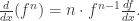
Definition. The derivative of f(x), denoted ${df}{dx}$ or just f'(x), is given by:

$f(x) = a_0 + a_1 x + a_2 x^2 + \ldots \implies \frac{df}{dx} = a_1 + 2a_2 x + 3a_3 x^2 + \ldots.$

Once again, the derivatives are formal derivatives, in the sense that we’re not thinking in terms of calculus and limits. Our derivative is merely a function which takes a polynomial and outputs another. The usual properties regarding derivatives of sums and products still hold.

$\frac{d}{dx}(f+g) = \frac{df}{dx} + \frac{dg}{dx}$ ;
$\frac{d}{dx}(fg) = f\frac{dg}{dx} + \frac{df}{dx}g$ ;
$\frac{d}{dx}(f^n) = n\cdot f^{n-1} \frac{df}{dx}.$

Do take note of the order of multiplication in the product law since the ring may well be non-commutative. Once again, the proof is left to the reader, but we’ll leave a hint to make his/her job easier. For the product law, note that the maps

$(f,g)\mapsto \frac{d}{dx}(fg)$ and $(f,g) \mapsto f\frac{dg}{dx} + \frac{df}{dx}g$

are both bilinear in f and g. In other words, if we fix f (resp. g), then the resulting map is linear in g (resp. f). This reduces to the case of monomials $f(x) = x^m$ , $g(x) = x^n$ .

Now, the next bombshell is: $\deg(\frac{df}{dx}) \ne \deg(f)-1$ in general, even for commutative rings, in fact, even for fields. Note that if the leading coefficient of f is $a_n x^n$ , then its derivative is $na_n x^{n-1}$ , which can be zero even if a_n ≠ 0.

E.g. let R = Z/3 which is a finite field. Then the polynomial $f(x) = x^3 + x^2 + 1$ has derivative $3x^2 + 2x = 2x$ since 3 = 3·1 = 0 in the ring R.

In general, we merely have $\deg(\frac{df}{dx}) \le \deg(f)-1$ .

Polynomials as Functions

Any student of elementary algebra knows that we can substitute values in x to evaluate a polynomial. This holds for $f(x) \in R[x]$ too.

Problem 1: product is not preserved if R is non-commutative.

We prefer not to do it when R is not commutative, because if we substitute x=r, then it’s not true in general that (fg)(r) = f(r)g(r).

E.g. consider the quaternion ring H. Suppose f(x) = ix and g(x) = jx. Then fg = (ij)x² = kx². This gives:

f(i) = -1, g(i) = –k but (fg)(i) = –k ≠ f(i)g(i).

The problem occurs because x=r does not commute with the coefficients of f(x), so we won’t attempt to interpret f as a function when the coefficients don’t commute.

Problem 2 : a non-zero polynomial can be a zero function.

This is best given by the example of R = Z/3. Take the polynomial f(x) = x³–x. The only elements of R are {0, 1, 2} mod 3, and all these satisfy f(0) = f(1) = f(2) = 0. More generally, if p is a prime, then the polynomial f(x) = x^p–x over the ring Z/p becomes the zero function by Fermat’s little theorem.

With those caveats out of the way, let’s state the main theorem of this section.

Theorem. Let R be a commutative ring. The evaluation map gives a ring homomorphism:

$R[x] \to \text{Func}(R, R), \ f(x) \mapsto (r \mapsto f(r)),$

where Func(R, R) is the set of functions R → R with addition and product given by: for all $f, g \in \text{Func}(R,R)$ ,

$(f+g)(r) = f(r)+g(r)$ ;

$(f\times g)(r) = f(r)g(r)$ .

The unity 1 is the constant function which takes all r to 1.

We’ve already seen that the evaluation map is not injective in general. Clearly, it’s also far from surjective.

Remainder Theorem

Throughout this section, let’s assume R is commutative.

Theorem. Let $f(x), g(x)\in R[x]$ , where g(x) is monic (recall: this means leading coeff = 1). Then we can write:

$f(x) = g(x)q(x) + r(x)$ ,

for some $q(x), r(x)\in R[x]$ such that deg(r) < deg(g) (this includes g=0, whose degree is -∞).

Furthermore, q(x) and r(x) are unique, and we them the quotient and remainder of f(x) ÷ g(x) respectively.

We’ll sketch the proof: which is almost identical to the case of secondary school algebra.

Case 1: deg(f) < deg(g). The only possibility is q(x)=0, r(x)=f(x), because if q≠0, then deg(gq) = deg(g)+deg(q) ≥ deg(g) > deg(r) (important: the first equality holds because g is monic!) which gives deg(f) = deg(gq+r) = deg(gq). But deg(gq) ≥ deg(g) so this contradicts the case assumption.
Case 2: deg(f) ≥ deg(g). Let $f(x) = a_n x^n + \ldots + a_0$ , where n = deg(f). Show that the leading coefficient of q(x) must be $g(x) = a_n x^{n-m} + \ldots$ , where m = deg(g). Then apply induction on deg(f).

In particular, suppose g(x) = x – c for some c in R. Then f(x) = q(x)(x – c) + r, where r is a constant. Substitute x=c to obtain f(c) = r, so we have:

Remainder Theorem. If $f(x)\in R[x]$ and $c\in R$ , then we have:

$f(x) = (x-c)q(x) + f(c)$ ,

for some $q(x)\in R[x]$ . As a corollary, we get the Factor Theorem : if f(c) = 0, then f(x) = (x-c)q(x) for some polynomial q(x).

[ An element c of R is called a root of f(x) if f(c) = 0. ]

Here’s another way of looking at it. Fixing c, we get a surjective ring homomorphism R[x] → R which takes f(x) → f(c). Then the factor theorem says the kernel of this map is precisely <x–c>.

Example 1

Consider the ring R[x, y, z] of all polynomials with real coefficients in x, y, z. This is (canonically isomorphic to) the ring of polynomials R[z], where R = R[x, y]. Now let (a, b, c) be an ordered triplet of real numbers.

The remainder theorem for R = R[x, y] gives us f(x, y, z) = (z–c)q(x, y, z) + r(x, y).
Applying remainder theorem to R = R[x] gives us r(x, y) = (y–b)q₂(x, y) + r₂(x).
Finally, applying it to R = R gives r₂(x) = (x–a)q₃(x) + r₃.

In conclusion:

$f(x,y,z) = (z-c)q(x,y,z) + (y-b)q_2(x,y) + (x-a)q_3(x) + r_3,$

and upon substituting x=a, y=b, z=c, we get r₃= f(a, b, c). In short, the ring homomorphism R[x, y, z] → R which takes f(x, y, z) to a real number by evaluating it at (a, b, c) has ideal I = <x–a, y–b, z–c>. Since the quotient R[x, y, z]/I is isomorphic to R by the first isomorphism theorem, I is maximal.

Example 2

Suppose R is an integral domain and $f(x)\in R[x]$ is of degree n. Denote the distinct roots of f by $r_1, r_2, \ldots, r_m$ . We shall prove that m ≤ n.

Indeed, since $f(r_m) = 0$ , by the Factor Theorem, $f(x) = g(x)(x - r_m)$ . Now for every other root, $r_i, 1 \le i \le m-1$ , we have $0 = f(r_i) = g(r_i)(r_i - r_m)$ . Since the r_i‘s are distinct, r_i–r_m ≠ 0. Since R is an integral domain, this implies $r_1, \ldots, r_{m-1}$ are also roots of g(x). Since deg(g) = deg(f) – 1, apply induction.

If R has zero-divisors, things can go very wrong. E.g. in R × R, the innocuous looking quadratic equation x²=x has 4 solutions: (0, 0), (0, 1), (1, 0) and (1, 1).

Omake: Shamir’s Secret Sharing Scheme

Polynomials in abstract ring theory are a key ingredient in Shamir’s secret sharing protocol. The problem is as follows: you have a secret code (e.g. 5-digit number) to a safe containing some highly sensitive documents. You’d like to distribute the code among 10 scientists so that:

any 3 scientists can cooperate and obtain the code, but
if any 2 scientists cooperate, they get absolutely no information on the code.

The second factor is critical: not only do the 2 scientists not know the full code, but the amount of knowledge they have pertaining to the code is zilch! In short, cutting up the code into binary bits and distributing them is out of the question, since each scientists would then know something about the code (each bit cuts the number of possibilities by half).

Shamir’s ingenious solution is as follows: pick a reasonably large prime p and take the finite field R = Z/p. Now:

The computer randomly picks a polynomial $f(x) = ax^2 + bx + c$ such that f(0) = c = secret code. The case of a=0 is not excluded.
For i = 1, 2, …, 10, the computer then calculates f(i) and sends it to scientist #i.
If any three scientists cooperate, they would have f(i), f(j), f(k) for three distinct positive integers i, j, k, and we know that every quadratic equation is uniquely determined by 3 points.
If two scientists cooperate to get f(i) and f(j), the amount of information they have on the code is still zilch since for every value of f(0), there is a unique solution for f.

Step 3 can be performed by the Lagrange interpolation formula if one so desires: to interpolate (i, f(i)), (j, f(j)) and (k, f(k)), compute:

$f(x) = f(i)\cdot\frac{(x-j)(x-k)}{(i-j)(i-k)} + f(j)\cdot\frac{(x-i)(x-k)}{(j-i)(j-k)} + f(k)\cdot\frac{(x-i)(x-j)}{(k-i)(k-j)},$

which is well-defined if i, j and k are distinct. Or we can solve simultaneous equations: e.g. to solve for f(1) = 2, f(2) = 3, f(3) = 9 for mod p=11, we have:

$\begin{matrix}a + b + c = 2\\ 4a + 2b + c = 3\\ 9a+3b+c = 9\end{matrix}\ \implies a = 8, b = 10, c=6\implies f(x) = 8x^2 + 10x+6$

so the secret code is 6.

In the general case, say, you wish to design a secret sharing system whereby any (n+1) scientists can collaborate to obtain the code, and any n scientists cannot figure out anything about the code. To that end, a polynomial of degree n is required. Once again, Lagrange’s interpolation formula allows us to recover the entire polynomial given (n+1) distinct points, and hence the secret code.

Posted in Notes | Tagged cryptography, derivatives, factor theorem, polynomials, remainder theorem, ring theory, secret sharing | Leave a comment

Introduction to Ring Theory (6)

Posted on October 27, 2012 by limsup

Let’s keep stock of what we’ve covered so far for ring theory, and compare it to the case of groups. There are loads of parallels between the two cases.

G is a group	R is a ring.
Abelian groups.	Commutative rings.
Group products.	Ring products.
$H\subseteq G$ is a subgroup.	$S\subseteq R$ is a subring.
Intersection of subgroups is a subgroup.	Intersection of subrings is a subring.

Next, we look at normal subgroups of a group and ideals of a ring.

Normal subgroups.	Ideals.
If N is normal in G, then G/N is a group quotient.	If I is an ideal of R, then R/I is a ring quotient.
Intersection of normal subgroups is a normal subgroup.	Intersection of ideals is an ideal.
If $H\subseteq G$ is a subgroup and N is a normal subgroup of G, then $H\cap N$ is a normal subgroup of H.	If $S\subseteq R$ is a subring and I is an ideal of R, then $S\cap I$ is an ideal of S.
If $H\subseteq G$ is a subgroup and $N\subseteq G$ is a normal subgroup, then HN is a subgroup of G	If $S\subseteq R$ is a subring and $I\subseteq R$ is an ideal, then I+S is a subring of R.
If $N_1, N_2\subseteq G$ are normal subgroups, then so is $N_1 N_2$ .	If $I_1, I_2\subseteq R$ are ideals, then so is $I_1 + I_2$ .
??	If $I_1, I_2\subseteq R$ are ideals, then so is $I_1 I_2$ .

Finally, there’re group and ring homomorphisms.

f : G → H is a group homomorphism.	f : R → S is a ring homomorphism.
Composing group homomorphisms gives a group homomorphism.	Composing ring homomorphisms gives a ring homomorphism.
If $K\subseteq G$ is a subgroup, then so is $f(K)\subseteq H$ .	If $T\subseteq R$ is a subring, then so is $f(T)\subseteq S$ .
If $L\subseteq H$ is a subgroup, then so is $f^{-1}(L)\subseteq G$ .	If $U\subseteq S$ is a subring, then so is $f^{-1}(U)\subseteq R$ .
If $N\subseteq H$ is a normal subgroup, then so is $f^{-1}(N)\subseteq G$ .	If $J\subseteq S$ is an ideal, then so is $f^{-1}(J)\subseteq R$ .
First isomorphism theorem: $G/\text{ker}(f)\cong \text{im}(f)$ as groups.	First isomorphism theorem: $R/\text{ker}(f)\cong \text{im}(f)$ as rings.
Second isomorphism theorem: let $H\subseteq G$ be a subgroup and $N\subseteq G$ be a normal subgroup. Then $H/(H\cap N)\cong HN/N$ .	Second isomorphism theorem: let $S\subseteq R$ be a subring and $I\subseteq R$ be an ideal. Then $S/(S\cap I) \cong (S+I)/I$ .
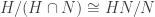Third isomorphism theorem: let $N\subseteq H\subseteq G$ , where N and H are normal subgroups of G. Then $(G/N)/(H/N) \cong G/H$ .	Third isomorphism theorem: let $I\subseteq J\subseteq R$ , where I and J are ideals of R. Then $(R/I)/(J/I) \cong R/J$ .

Posted in Notes | Tagged group theory, groups, ring theory, rings, summary | Leave a comment

Introduction to Ring Theory (5)

Posted on October 25, 2012 by limsup

Our first order of the day is to state the correspondence between the ideals and subrings of R/I and those of R. This is totally analogous to the case of groups.

Theorem. Let I be an ideal of R. There are 1-1 correspondences:

$\begin{aligned}\{ S : I\subseteq S \subseteq R, S\text{ subring of } R\} &\leftrightarrow\{ T : T \text{ subring of } R/I\} \\ \{ J : I\subseteq J \subseteq R, J\text{ ideal of } R\} &\leftrightarrow \{ K : K \text{ ideal of } R/I\}\end{aligned}$

which preserve inclusion: i.e. $S\subseteq S'$ on the LHS if and only if $T \subseteq T'$ on the RHS. The same holds for the ideals.

[ Correspondence for the lattices of ideals and subrings between those of R (containing I), and those of R/I. In general, an ideal can be contained in a subring, but not vice versa, unless the ideal is the whole ring R (why?). ]

Sketch of Proof.

The proof is similar to the case of groups. For A such that $I \subseteq A \subseteq R$ is an ideal or subring of R, let the corresponding element on the RHS be A/I. If A is an ideal (resp. subring) of R, then A/I is an ideal (resp. subring) of R/I.

Conversely, if $B\subseteq R/I$ is a subring or ideal, then let the corresponding A on the LHS be $A = f^{-1}(B)$ . Prove that A contains I and A/I = B. Now fill up the proof by showing that by composing these two arrows in either order, we get the identity map on either the LHS or RHS. ♦

Corollary

The above correspondence preserves intersections and sums of ideals, but not products.

Proof.

Suppose we have ideals $J_i \supseteq I$ on the LHS, indexed by i. Each ideal then corresponds to $J_i/I$ on the RHS.

Intersection. From the lattice structure on the LHS, $J = \cap_i J_i$ is the largest ideal (containing I) such that $J\subseteq J_i$ for each i. Translating it to the RHS, the corresponding J/I is also the largest ideal which contained in all $J_i/I$ . Hence $J/I = \cap_i J_i/I$ . This is yet another example of a “universal proof” we alluded to earlier.
Sum. Similar to intersection, except now we’re dealing with the smallest ideal containing every $J_i$ .
Product. See the following example (the gist is that even if $I_1, I_2\supseteq I$ , their intersection may not contain I).

Examples

Let 12Z be an ideal in Z, which gives the quotient ring Z/12. Now the ideals of Z which contain 12Z correspond to the positive divisors of 12, so we have Z, 2Z, 3Z, 4Z, 6Z, 12Z. These give corresponding ideals of Z/30: <1>, <2>, <3>, <5>, <6>, <10>, <15>, <30>. E.g. the ideal <5> = {0, 5, 10, 15, 20, 25} modulo 30.

Intersection on the LHS gives $4\mathbf{Z}\cap 6\mathbf{Z} = 2\mathbf{Z}$ which corresponds to <4> ∩ <6> = <2> on the RHS.
Product on the LHS gives 4Z × 6Z = 24Z which doesn’t contain 12Z, so it doesn’t correspond to anything on RHS.

Consider the homomorphism R[x, y] → R[x], where R[x, y] (resp. R[x]) is the ring of all polynomials in x, y (resp. x) with real coefficients. The homomorphism is given by f(x, y) → f(x, 0). It’s quite easy to show that the ideal is I = <y>, the set of all multiples of y. So we have an isomorphism f : R[x, y]/<y> → R[x].
- Consider the subring R of R[x]. This corresponds to the pullback $f^{-1}(\mathbf{R}) = \mathbf{R} + \left<y\right> \subset \mathbf{R}[x,y]$ , which has basis given by 1, together with x^myⁿ, where m ≥ 0 and n > 0.
- Consider the subring R[x²] of R[x], which comprises of polynomials whose terms are all even powers of x. The pullback gives a subring of R[x, y] which has basis given by x^myⁿ, where n > 0, or (m, n) = (2k, 0) for some non-negative integer k.

Case of Commutative Rings

Let’s assume our R is commutative now. We wish to derive conditions for the ring quotient R/I to be an integral domain or a field. First, a result:

Proposition. A commutative ring R≠{0} is a field if and only if it has only two ideals: {0} and itself.

Proof.

We already know that a division ring has no non-trivial ideals. For the converse, suppose R has only two ideals {0} and itself. Let $x\in R-\{0\}$ . Then <x> is an ideal which is non-zero, hence <x>=R. This implies 1 is contained in <x>, so there exists an element y in R such that xy = 1. ♦

It is not true that a (possibly non-commutative) ring R ≠ {0} is a division ring if and only if it has only two ideals. For a counter-example, the ring of n × n real matrices has no non-trivial ideals (which we’ll see in a later post). If n > 1, this is clearly not a division ring.

Theorem. Let R be a commutative ring and I ≠ R be an ideal.

R/I is an integral domain if and only if $a, b\in R, ab\in I \implies a\in I \text{ or } b\in I$ . We call such an I a prime ideal.

R/I is a field if and only if there is no ideal J of R, $I\subsetneq J\subsetneq R$ , i.e. no ideal is strictly contained between I and R. We call such an I a maximal ideal.

Proof. For (1), saying R/I is an integral domain means

$(a+I)(b+I) = 0+I \implies a+I=0+I \text{ or } b+I=0+I$ .

Unravelling the definition, this is equivalent to saying $ab\in I \implies a\in I\text{ or }b\in I$ .

For (2), by the proposition above, R/I is a field if and only if its only ideals are {0} and itself. By the correspondence theorem above, this is equivalent to saying the only ideals J, $I\subseteq J \subseteq R$ are J=I or J=R. ♦

Examples

Consider Z again. Its only ideals are nZ, where n ≥ 0.
1. If n=0, then {0} is a prime ideal which is not maximal.
2. If n=1, then <1> = Z is neither prime nor maximal, by definition.
3. For n>1, whenever n is composite, Z/n is not an integral domain; but if n is prime, Z/n is a field. This shows that nZ is prime iff nZ is maximal iff n is prime.
Take the ring R[x, y], set of polynomials in x, y with real coefficients. For any real numbers a and b, consider the ideal I = <x–a, y–b>. Replacing x → x–a and y → y–b, it’s easy to see any f(x, y) can be written in the form $f(x,y) = (x-a)k_1(x,y) + (y-b)k_2(x,y) + c\in I+c$ for some real c. Hence R[x, y]/I is isomorphic to R and I is maximal.
On the other hand, take the ideal I = <y>. We saw earlier that R[x, y]/I is isomorphic to R[x] which is an integral domain but not a field. Hence, <y> is a prime ideal which is not maximal. Indeed, <y> is strictly contained in <x, y> so of course it’s not maximal.

Chinese Remainder Theorem

Throughout this section, let I and J be ideals of a commutative ring R. Consider the natural map R → (R/I) × (R/J) via projecting r to (r+I, r+J). Clearly the kernel comprises of all r in both I and J, i.e. ker = I ∩ J. By the first isomorphism theorem, we get a monomorphism:

$R/(I\cap J) \hookrightarrow (R/I) \times (R/J).$

Now assume I ∩ J = {0}, i.e. we get a monomorphism R → (R/I) × (R/J). The question we want to devote ourselves to is:

When’s R → (R/I) × (R/J) an isomorphism?

To make our lives ahead easier, let us define some new notation.

Definition. If I is an ideal of R, and a, b are arbitrary elements of R, we write a ≡ b (mod I) to mean $a-b\in I$ . Since I is an additive subgroup, we see that this is an equivalence relation. Further:

if a ≡ b (mod I) and c ≡ d (mod I), then a+c ≡ b+d (mod I) and ac ≡ bd (mod I).

The proof for these properties is identical to that for the corresponding properties of modular arithmetic.

Back to the question.

For R → (R/I) × (R/J) to be an isomorphism, there must be an $x\in R$ which maps to (0, 1), i.e. x ≡ 0 (mod I) and y ≡ 1 (mod J). By the same token, we get y such that y ≡ 1 (mod I) and y ≡ 0 (mod J). But now look at x+y. We have x+y ≡ 1 (mod I) and (mod J), so x+y ≡ 1 (mod I∩J). Since I∩J = {0}, x+y=1.

Thus the ideal I+J contains 1, and must be the whole ring R! This condition turns out to be sufficient too.

Definition. If I, J are ideals of R such that I+J = R, then the two ideals are said to be coprime. [ This is motivated by the fact that in Z, ideals mZ + nZ = Z iff (m, n) = 1. ]

Chinese Remainder Theorem. If I, J are coprime ideals of R such that I ∩ J = {0}, then R → (R/I) × (R/J) is an isomorphism.

Proof.

It suffices to show the map is surjective. The process is essentially the reverse of the above. Since I+J contains 1, pick $x\in I, y\in J$ , x+y = 1. Taking this expression mod I and J, we get x ≡ 1 (mod J) and y ≡ 1 (mod I). In a nutshell:

$x\equiv 0 \pmod I, \ x\equiv 1\pmod J,\quad y\equiv 1\pmod I, \ y\equiv 0\pmod J.$

Now for any a, b in R, the element bx+ay maps to a mod I and b mod J respectively. This shows that R → (R/I) × (R/J) is an isomorphism. ♦

Example

Consider the ring Z/35, with ideals I=<7> and J=<5>. Then the above conditions are satisfied:

I ∩ J = {0} since the only integers divisible by 7 and 5 are multiples of 35;
I+J = Z/35 since 21 + 15 ≡ 1 (mod 35), i.e. there exist $x\in I, y\in J$ , x+y=1.

By the above theorem, we get an isomorphism

$\mathbf{Z}/35 \cong \mathbf{Z}/I \times \mathbf{Z}/J \cong \mathbf{Z}/7 \times \mathbf{Z}/5,$

which is the classical Chinese Remainder Theorem for number theory. Furthermore, the above proof gives us a concrete method of constructing a solution to $n\equiv a\pmod 7$ , $n\equiv b\pmod 5$ : just take n = ay+bx = 15a + 21b.

Posted in Notes | Tagged advanced, chinese remainder theorem, ideals, maximal ideals, prime ideals, ring theory, rings | Leave a comment

Introduction to Ring Theory (4)

Posted on October 23, 2012 by limsup

It’s now time to talk about homomorphisms.

Definition. Let R, S be rings. A function f : R → S is a ring homomorphism if it satisfies the following:

f(1_R) = 1_S;

f(x+y) = f(x) + f(y) for all x, y in R;

f(xy) = f(x) f(y) for all x, y in R.

Some immediate properties:

The second condition tells us f is a homomorphism of the underlying additive groups.
The first condition is not superfluous: consider the map R → R × R which takes x to (x, 0). This map satisfies the second and third conditions but not the first.
The first and third conditions tell us that units are taken to units, since if x is a unit, then xy = 1, so f(x) f(y) = f(1) and f(x) is also a unit. This helps to explain why we need the first condition: so that units go to units under a homomorphism.

However, zero-divisors don’t go to zero-divisors in general. For example, consider the map R × R → R which takes (x, y) to x. Then (1, 0) is a zero-divisor but the image, 1, is not.

One particularly important homomorphism is the projection R → R/I, for an ideal I of R, which takes x to x+I.

Needless to say, composition of two homomorphisms is also a homomorphism. One also defines a monomorphism (resp. epimorphism, isomorphism) to be an injective (resp. surjective, bijective) homomorphism.

Effect on Subrings and Ideals

Let’s examine the effect of f and its inverse on subrings and ideals.

Theorem. Let f : R → S be a ring homomorphism. Then:

if R’ is a subring of R, then f(R’) is a subring of S;

if S’ is a subring of S, then f^-1(S’) is a subring of R;

if J is an ideal of S, then f^-1(J) is an ideal of R;

if I is an ideal of R, then f(I) is not an ideal of R in general.

The first three statements are easy to prove: once again, they illustrate the general philosophy that the “pullback” f^-1 is better behaved that the “pushforward” f. We already saw this earlier with normal subgroups of groups. To obtain a counter-example for the fourth statement, take the inclusion map Z → Q. Then 2Z is an ideal in Z but clearly not an ideal in Q. [ Since Q is a field, its only ideals are 0 and itself. ]

In particular, we have the following special cases.

Definition. If f : R → S is a ring homomorphism, then f(R) = im(f) is the image of f; this is a subring of S. On the other hand, f^-1({0}) = ker(f) is the kernel of f; this is an ideal of R.

First Isomorphism Theorem

The three isomorphism theorems are strongly reminiscent of the case for groups.

First Theorem of Isomorphism. If f : R → S is a ring homomorphism and I = ker(f), then this induces an isomorphism φ:R/I → im(f)$ where φ(r+I) = f(r).

The proof is straight-forward: by the case for group theory, we already know that φ is an isomorphism of the additive groups. Clearly, it takes 1 to 1. To show it preserves product:

φ((r+I)(s+I)) = φ(rs+I) = f(rs) = f(r)f(s) = φ(r+I)φ(s+I).

One application of the theorem: suppose we wish to prove that if S is a subring of R, and I is an ideal of R, then S ∩ I is an ideal of S. Indeed, the composed homomorphisms S → R → R/I has kernel $\{s\in S: s+I = 0\} = S\cap I$ . Hence, the kernel of this map, S ∩ I, is an ideal of S and we get an injection S/(S ∩ I) → R/I.

Another useful application: suppose we wish to prove that I is an ideal of R and $R/I\cong S$ , where I, R and S are explicitly defined. An easy way to do this is via constructing an epimorphism R → S with kernel I and letting the first isomorphism theorem do its job. Here’s a concrete example.

Example

Let’s take an example in the previous post, where U is the ring of 2 × 2 upper-triangular real matrices $\begin{pmatrix}* & *\\{0}& *\end{pmatrix}$ . Map f : U → R×R by taking the two diagonal entries a, b to the ordered pair (a, b). Then f is an epimorphism so we get

$\mathbf{R}\times\mathbf{R} \cong U/\text{ker}(f),$

where I = ker(f) is the set of all strictly upper-triangular real matrices $\begin{pmatrix}{0}&*\\{0}&{0}\end{pmatrix}$ .

Second + Third Isomorphism Theorems

In preparing for the second isomorphism theorem, let’s prove that if S is a subring of R and I is an ideal of R, then S+I is a subring of R. Indeed, S+I is an additive subgroup of R, so it suffices to show that it’s closed under multiplication, but this follows from:

$x_1, x_2\in S, y_1, y_2\in I \implies (x_1 + y_1)(x_2 + y_2) = \overbrace{x_1 x_2}^{\in S} + \overbrace{x_1 y_2 + y_1 x_2 + y_1 y_2}^{\in I}.$

Another way of proving this would be:

$(S+I)(S+I) = \overbrace{S^2}^{\subseteq S} + \overbrace{SI + IS + I^2}^{\subseteq I}\subseteq S + I.$

The second method is actually “preferred” since it’s more concise: the reader is urged to get comfortable with that kind of notation. Just a reminder: the product AB of two sets here refers to the set of all finite sums $\sum_{i=1}^n x_i y_i$ , with $x_i\in A, y_i\in B$ .

Second Isomorphism Theorem. Let $S\subseteq R$ and $I\subseteq R$ be a subring and an ideal respectively. We already know that $S+I \subseteq R$ is a subring and $I\cap S\subseteq S$ is an ideal of S. Then:

$S/(S\cap I) \cong (S+I)/I$ .

Once again, by the second isomorphism theorem for groups, we already have an isomorphism of additive groups. So it remains to consider whether the map preserves the unity “1” and the product of two elements. But the map takes s+(S ∩ I) on the LHS to s+I on the RHS. Thus it’s easy to verify that the map takes “1” to “1”, and preserves the product.

Finally, to prepare for the last isomorphism theorem, consider $I\subseteq J \subseteq R$ , where I and J are ideals of R. Then the additive group quotient J/I is an ideal of R/I, because every element of J/I can be written as x+I for some x in J. Thus the products (x+I)(r+I) = xr+I and (r+I)(x+I) = rx+I are both elements of J/I since xr and rx are in J.

Third Theorem of Isomorphism. Let $I\subseteq J \subseteq R$ where I and J are ideals of R. Then we have an isomorphism of rings:

$(R/I) / (J/I) \cong R/J$ .

Same proof: by the results of group theory, we already know the underlying additve groups are isomorphism. To show isomorphism as rings, it remains to show 1 maps to 1, and product on the LHS maps to product on the RHS, which is quite easy.

Posted in Notes | Tagged homomorphism, isomorphism theorems, kernels | Leave a comment

Introduction to Ring Theory (3)

Posted on October 20, 2012 by limsup

Ideals and Ring Quotients

Suppose I is a subgroup of (R, +). Since + is abelian, I is automatically a normal subgroup and we get the group quotient (R/I, +). One asks when we can define the product operation on R/I.

To be specific, each coset in R/I is of the form (r+I), for some r in R. We wish to define the product operation on R/I via (r+I)(s+I) := rs+I. The question arises as to whether the operation is well-defined, i.e.

If r+I = r’+I and s+I = s’+I, then is it true that rs+I = r’s’+I ?

Now, r+I = r’+I iff $r-r' \in I$ . So we need the condition:

$r-r', s-s' \in I \implies rs-r's'\in I.$

But then we have:

$rs - r's' = r\overbrace{(s-s')}^{\in I} + \overbrace{(r-r')}^{\in I}s'.$

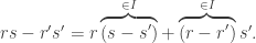
Letting r = r’ and s’ = 0, we get the condition $s\in I \implies rs\in I$ for each r in R. Likewise, in letting s = s’ and r’ = 0, we get 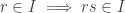$r\in I \implies rs\in I$ for each s in R. Clearly, these conditions suffice to ensure that the above hold.

Definition. An (two-sided) ideal of R is an additive subgroup I of (R, +) such that $r\in R, s \in I \implies rs, sr\in I$ . Note that if R is commutative, then rs=sr so it suffices to check for $rs\in I$ .

From the above reasoning, an ideal I of R gives a ring quotient R/I which is the set of all cosets r+I, with additional and multiplication given by (r+I)+(s+I) := (r+s)+I and (r+I)(s+I) = (rs)+I. The corresponding unity is given by 1+I.

Examples

Every additive subgroup of the ring Z is of the form nZ, where n ≥ 0. It’s clear that this is an ideal. For n=0, we have Z/{0} = Z. Otherwise, n>0 and Z/nZ is precisely the ring of integers mod n, which we had denoted by Z/n.
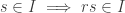
Let R be a division ring. Certainly, {0} and R are ideals, with respective quotients R and the trivial ring. Conversely, suppose I is an ideal of R which contains x≠0. Then x is a unit so there exists a y in R such that xy=1. So $1 = xy \in I$ by definition of ideal. But this means for any r in R, $r = 1\cdot r \in I$ , i.e. I = R. This means a division ring has no non-trivial ideals. In particular, a field has no non-trivial ideal.
The ring of 2 × 2 real matrices has no non-trivial ideal too. This will follow from a later chapter on matrix rings.
If U denotes the ring of 2 × 2 upper-triangular real matrices $\begin{pmatrix} * & *\\ 0 & *\end{pmatrix}$ , then the subset I of strictly upper-triangular real matrices $\begin{pmatrix} 0 & *\\ {0}& 0\end{pmatrix}$ is an ideal since $\begin{pmatrix}0 & *\\{0}&0\end{pmatrix}$ $\begin{pmatrix}* & *\\{0}& *\end{pmatrix}$ = $\begin{pmatrix}0 & *\\{0}& 0\end{pmatrix}$ and similarly $\begin{pmatrix}* & *\\{0} & *\end{pmatrix}$ $\begin{pmatrix} 0 & * \\ {0} & 0\end{pmatrix}$ = $\begin{pmatrix}0 & *\\{0} & 0\end{pmatrix}$ . The ring quotient U/I is isomorphic to R × R by mapping the two diagonal entries (a and b) of a matrix to $(a,b)\in\mathbf{R}\times\mathbf{R}$ .
In the ring R × R, the only ideals are {(0, 0)}, {0} × R, R × {0} and R × R. This follows from the following.
1. If R and S are rings, then all ideals of R × S are of the form I × J, where I, J are respectively ideals of R, S.
2. Is it true that all subrings of R × S are of the form T × U, where T, U are respectively subrings of R, S?
Every ideal of R[x] is of the form <p(x)>, the set of multiples of p(x), where p(x)=0 or p(x) is a monic polynomial. This will follow from a later chapter on polynomial rings. This is not true for Z[x]: for example, the set $\{2a(x) + x\cdot b(x) : a(x), b(x) \in \mathbf{Z}[x]\}$ is an ideal which is not of the above form.

Operations on Ideals

The following are a list of common operations on ideals. Their proofs are easy and left as exercises.

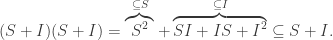
Addition. If I and J are ideals of R, let $I+J=\{x+y : x\in I, y\in J\}$ . This is an ideal of R. In fact, it is the “smallest ideal of R containing I and J“. [ This just means (i) it contains both I and J, and (ii) any ideal containing I and J must contain it. ]
Intersection. If {I_i} is a collection of ideals of R, then so is the intersection I = ∩_iI_i.
Product. If I and J are ideals of R, let $IJ = \{x_1 y_1 + \ldots + x_n y_n : x_i\in I, y_i \in I\}$ . Then IJ is an ideal of R.

A few words about the product, since the reader may not be accustomed to it. Note that we only allow finitely many terms in the sum, although the number of terms has no upper-bound. Also, this differs from the “pairwise products” which one may be inclined to define via $S=\{xy : x\in I, y\in J\}$ .

Exercise.

Consider the ring of integers Z. As stated above, each ideal is of the form mZ, where m is a non-negative integer. Determine the ideals mZ + nZ, mZ ∩ nZ and mZ·nZ by describing them in terms of number-theoretic operations on integers.

Answer (highlight to read): [ Addition, intersection and product of ideals correspond to the lowest common multiple, greatest common divisor and product of the corresponding non-negative integers. ]

Generated Ideals

Now, since the intersection of ideals is an ideal, let’s define the generated ideal as before.

Definition. Let X be an arbitrary subset of R. The intersection of all ideals containing X is denoted by <X> and is called the ideal generated by X.

By now, you should have seen the term “generated by” many times and have a good idea what that means. Under this definition, the product of ideals IJ is simply the ideal generated by the set of pairwise products: $S=\{xy : x\in I, y\in J\}$ .

What does the ideal <X> look like? For one thing, it must contain every x of X, and hence by definition of ideals, it contains rxs for any $r, s\in R$ . Since <X> is closed under addition, it must contain all finite sums of the form $r_1 x_1 s_1 + \ldots r_n x_n s_n$ , where $x_i \in X$ and $r_i, s_i \in R$ . On the other hand, the set of all such elements clearly satisfies the conditions of being an ideal. Thus:

$\left<X\right> = \{r_1 x_1 s_1 + \ldots + r_n x_n s_n : x_i \in X, r_i, s_i \in R\}.$

Note that the x_i‘s are not necessarily distinct, since there’s no generic way to simplify $r_1 x s_1 + r_2 x s_2$ any further. However, if R is commutative, then we only need to consider:

$\left<X\right> = \{r_1 x_1 + \ldots + r_n x_n: x_i \in X, r_i\in R\}$

and the x_i‘s may be take to be distinct since $r_1 x + r_2 x = (r_1 + r_2)x$ . In particular,

for a singleton set X={x}, $\left<x\right> = \{rx : r\in R\}$ (for notational convenience, we set <x> := <{x}>) – such ideals are called principal ideals;
for two-element set X={x, y}, $\left<x,y\right> = \{rx + sy : r,s\in R\}$ ;
etc etc.

Examples (all commutative)

Let’s pick R[x]. Then the ideal <f(x)> is the set of all multiples of f(x).
Again pick R[x]. Consider the ideal I = <x²-1, x³-1>. A priori, it’s generated by two elements. Now is it principal (i.e. generated by one element)? The answer is yes. In fact, we claim I = <x-1>. Indeed: since x²-1 and x³-1 are both multiples of x-1, clearly I is contained in <x-1>. Conversely, x-1 = (x³-1) – x(x²-1) is an element of I. So <x-1> is contained in I. This completes our proof. [ Note: we’ll see later that every ideal of this ring is principal. This will have important consequences. ]
Pick Z[x]. Consider the ideal I = <2, x-1>. Is it principal? If it were, then we would have a polynomial f(x) such that <2, x-1> = <f(x)>. Since 2 is an element of <f(x)> it is a multiple of f(x). This can only happen if f(x)=-2, -1, 1 or 2, none of which works. So I is not a principal ideal in Z[x].
Pick the ring of Gaussian integers Z[i] from the previous post and take the ideal I = <8+i, 5-14i>. Is this ideal principal? Now that’s a little tricky: but it turns out it is! We claim I = <2-3i>. Indeed: since 8+i = (2-3i)(1+2i) and 5-14i = (2-3i)(4-i) are both multiples of 2-3i, I must be contained in <2-3i>. Conversely, 2-3i = 2(8+i) – i(5-14i) is an element of I, so <2-3i> is contained in I. Thus, I is principal! The reader may wonder how one can compute such relations effectively. This will be covered in a later post. [ We’ll also see that every ideal of Z[i] is principal, which marks the birth of algebraic number theory. ]

Posted in Notes | Tagged advanced, gaussian integers, generated ideals, ideals, principal ideals, ring quotients, ring theory | Leave a comment

Introduction to Ring Theory (2)

Posted on October 18, 2012 by limsup

Subrings

Just like groups have subgroups, we have:

Definition. A subset S of a ring R is a subring if it satisfies the following:

$1\in S$ ;

$r,s \in S \implies r-s\in S$ ;

$r,s\in S \implies rs\in S$ .

The first two conditions imply that S is a subgroup of (R, +). Together with the third condition, this means S inherits a ring structure from (R, +, ×) via the same addition and product operations. Clearly, if T is a subring of S which is in turn a subring of R, then T is a subring of R.

Examples

The ring of integers Z has no proper subring: since a subring must contain 1, it must contain all integers. Same goes for Z/n for positive integer n.
We have the sequence of subrings $\mathbf{Z} \subset \mathbf{Q} \subset \mathbf{R} \subset \mathbf{C}$ .
In the ring of 2 × 2 real matrices, the set U of upper-triangular matrices $\begin{pmatrix} * & * \\ 0 & *\end{pmatrix}$ forms a subring, and the set D of diagonal matrices forms a subring of U. [ Note that D is isomorphic to R × R, under component-wise addition and multiplication. We haven’t defined isomorphism, but you know what it means. 🙂 ]
In the ring of quaternions, the subset of elements of the form a+bi is a subring which is isomorphic to C. Thus, we have a commutative subring of a non-commutative ring. Specifically, we have a division ring with a subring which forms a field.
In the ring R × R, the subset {(r, r) : r in R} is a subring which is isomorphic to R.
In the ring of polynomials R[x], take the subset R[x²] comprising of polynomials whose terms are all even powers of x. This is a subring.

In the ring R × R, the subset R × {0} is not a subring, because it doesn’t contain the unity (1, 1). The reader may object that this ought to be a bona-fide subring since it’s isomorphic to R which is a ring with unity, but we wish to maintain consistency with the definition. In other words, what we have here is a “subrng” which is isomorphic to a ring, but still not a subring.

Incidentally, some books do not require a ring to possess a unity 1, in which case R × {0} would become a subring of R × R. Both rings would then have unities but the two unities are different elements. This can lead to much grief if we weren’t careful, which is why we would rather not deal with that case.

Generated Subrings

Basic property: the intersection of subrings is also a subring. Explicitly, if {S_i} is a collection of subrings of R, then ∩_iS_i is also a subring of R. The proof is standard:

Since 1 is in each S_i, it also lies in all ∩_iS_i.
If x, y are in ∩_iS_i, then they are in S_ifor all i; since each S_iis a subring, x–y lies in S_i, and so x–y lies in ∩_iS_itoo.
For multiplication, same as above, but replace x-y with xy. ♦

If X is an arbitrary subset of R, we let <X> be the intersection of all subrings of R which contain X. As in the case of groups, <X> is a subring of R containing X, and conversely any subring S of R containing X must contain <X>. We call this the subring of R generated by X.

Consider the field C of complex numbers. What’s the subring S generated by the empty set? Well S must contain 1, so since S is closed under addition it must also contain all integers. On the other hand, the set of all integers itself is already a subring. So S = Z.
Take the field C of complex numbers again. What’s the subring S generated by a single element 1/2? As before S must contain all integers. But now S must also contain all powers of 1/2 since it’s closed under multiplication. Therefore S contains all elements of the form a/2^m, where a is an integer and m is a non-negative integer. On the other hand, the set of all such elements forms a subring. So $S= \{a/2^m : a \in\mathbf{Z}, m\in\mathbf{Z}, m\ge 0\}$ .
Again take C. What’s the subring S generated by a single element i (i.e. √-1)? Now S contains all integers and also contains i. So it must contain all numbers of the form a+bi, where a, b are integers. Numbers of this form are called Gaussian integers. It’s clear that the set of Gaussian integers forms a subring, so S = set of Gaussian integers, denoted by Z[i].
Once again, take C. What’s the subring S generated by a single element π? Since S contains Z and π, and S is closed under addition and multiplication, S must contain all real numbers of the form $a_0 + a_1 \pi + \ldots + a_n \pi^n$ , $a_i\in\mathbf{R}$ . On the other hand, the set of such numbers clearly forms a subring, so S = set of all numbers of the form $\sum_{i=0}^n a_i \pi^n$ . Furthermore, it is known that π is transcendental, so different expressions give distinct numbers. To be specific, there is an isomorphism Z[x] → S, mapping x to π.
Now take R[x]. What’s the subring S generated by x²? Again S contains Z and the element x² so it must contain all polynomials in x² with integer coefficients. This means S = Z[x²]. On the other hand, we can also ask for the subring generated by R and x². This just means the subring generated by $\mathbf{R}\cup\{x^2\}$ . Now it’s clear that the resulting subring is R[x²].

Exercise. Consider the ring of all 2 × 2 real matrices.

Describe the subring generated by $\begin{pmatrix} 2 & 1\\ 1 & 2\end{pmatrix}$ .
Describe the subring generated by $\begin{pmatrix} 1 & 1\\{0} & 1\end{pmatrix}$ .
Describe the subring generated by both $\begin{pmatrix} 2 & 1\\ 1 & 2\end{pmatrix}$ and $\begin{pmatrix} 1 & 1\\{0} & 1\end{pmatrix}$ .

Posted in Notes | Tagged generated subrings, ring theory, rings, subrings | Leave a comment

Introduction to Ring Theory (1)

Posted on October 16, 2012 by limsup

Recall that in groups, one has only a binary operation *. Rings are algebraic structures with addition and multiplication operations – and consistency is ensured by the distributive property.

Definition. A ring R is a set together with two binary operations: (R, +, ×), satisfying the following properties.

(R, +) is an abelian group, with identity 0 and inverse of r denoted by -r.

(R, ×) satisfy the following:

(identity) there exists 1 in R (called the unity) such that 1×r = r×1 = r;

(associative) for any r, s, t in R, we have (r×s)×t = r×(s×t).

(Distributive) We have r×(s+t) = (r×s)+(r×t) for any r, s, t in R.

In general, multiplication in a ring need not commute, i.e. xy ≠ yx in general. If xy=yx, then we say the ring is commutative.

The first order of the day is to prove the following very basic properties:

0×r = r×0 = 0 for any r;
(-r)×s = -(r×s) = r×(-s) for any r and s.

Quick proof

To show r×0 = 0, use the distributive property: r×0 + r×0 = r×(0+0) = r×0. So adding -(r×0) to both sides proves r×0 = 0.
To show -(r×s) = r×(-s), we use the distributive property again: r×(-s) + r×s = r×((-s)+s) = r×0 = 0. ♦

Following our intuition from elementary algebra, we use the following notations/conventions.

r×s is denoted as rs for short.
For a positive integer n, product of n terms of r is denoted by $r \times r\times \ldots \times r = r^n$ . Also, $r^0 = 1$ .
a+(-b) is denoted as a–b for short. Thus we have (a–b)c = (a+(-b))c = ac+(-b)c = ac+(-(bc)) = ac–bc by the above.
Product is always performed before addition.

Various conventions exist in different literature. For example, some books like Herstein’s Topics in Algebra or Hungerford’s Algebra (GTM 73) define a ring without the condition of the existence of unity (1). Thus by their definition, 2Z (the set of even numbers) forms a ring under the usual addition and multiplication. Whichever is preferred is a matter of taste, but we’ll stick to our version above, under which Z is a ring but 2Z is not. If we ever need to talk about rings without identity, we’ll call them rngs instead (rings without “i”dentity).

Anyone who’s done matrix arithmetic knows that rings come in all kinds of flavours. Let’s go through some technical definitions here below.

Definitions. Let R be a ring. First we look at the elements of R.

A zero-divisor is an element x, such that there exist non-zero y, z for which xy = zx = 0.

A unit is an element x, such that there exist y, z for which xy = zx = 1. Here, we must have y=z since y = (zx)y = z(xy) = z. We usually denote $y = x^{-1}$ .

Now let’s look at the whole ring R.

A trivial ring is where 1=0. If so, any r = r×1 = r×0 = 0, so there’s only 1 element: {0}.

If every non-zero element of the non-trivial ring R is a unit, we call the ring a division ring.

If R is a non-trivial commutative ring, and $xy = 0 \implies x=0 \text{ or } y=0$ , then we call the ring an integral domain (or just domain if we’re lazy).

A commutative division ring is called a field.

[ Another way of looking at fields: a field is a an algebraic structure where (R, +) is an abelian group, (R-{0}, ×) is an abelian group, and the distributive law holds. ] The reason we wish to exclude trivial rings in some of the above definitions, is akin to why we’d exclude 1 as a prime number. That being said, there’re people who’re interested in studying structures over the field with 1 element (for very deep reasons), but that’s another story for another day.

Examples

We hope that the reader is not put off by the large number of technical definitions above. If in doubt, feel free to ignore some of them, since we won’t be using them for now.

The integers Z form an integral domain under the usual addition/product, but not a field since 2 is not a unit.
The rationals Q, reals R, and complex numbers C each form a field since every non-zero element can be inverted.
The set of integers modulo prime p, given by Z/p, forms a field under addition and product mod p.
The set of integers modulo composite n, given by Z/n, forms a commutative ring but is not an integral domain or field. E.g. in Z/6, 2×3 = 0.
The set of 2×2 matrices with real entries forms a non-commutative ring. There are lots of examples of zero-divisors, e.g. $\begin{pmatrix}1 & -1\\ 1 & -1\end{pmatrix} \times \begin{pmatrix} 1 & 1 \\ 1 & 1\end{pmatrix}$ = $\begin{pmatrix}0 & 0\\{0}&0\end{pmatrix}$ = $\begin{pmatrix}1 & 1\\1 & 1\end{pmatrix}\begin{pmatrix}1 & 1\\-1 & -1\end{pmatrix}$ .
The set of quaternions is $\mathbf{H} = \{a+bi + cj + dk : a,b,c,d \in \mathbf{R}\}$ , where i, j, k satisfy the multiplication laws $i^2 = j^2 = k^2 = -1$ and ij = –ji = k, jk = –kj = i, ki = –ik = j. Then H is a non-commutative division ring – if you’re not familiar with quaternions, just take it as it is for now.
The set $\mathbf{R}\times\mathbf{R} = \{(x,y) : x, y\in\mathbf{R}\}$ of ordered pairs of real numbers is a ring under component-wise addition and multiplication. This is not an integral domain since (1, 0) × (0, 1) = (0, 0).
The set of polynomials in x with real coefficients, R[x], is an integral domain. It is not a field since x is not a unit. Likewise, the set Z[x] of polynomials in x with integer coefficients is an integral domain.

Exercises

Does the set of 3-vectors (x, y, z) form a ring under vector addition and scalar product? What about vector addition and cross product?
For each of the above examples, describe the set of units.
Take R, the set of real numbers, with the following operations: r # s = r + s + 1, r * s = rs + r + s. Does this form a ring under # and * ? What are the identity and additive inverse of r?
We can generalise example 7 as follows. Given rings R and S, prove that R × S is a ring under component-wise addition and multiplication.

Intuition

Here’re some instances where one has to be careful with intuition.

(1) “Cancellation” only works if the value cancelled is not a zero-divisor.

For example, if ac = bc, it would be too rash to say if c ≠ 0, then a=b. On the other hand, if c is not a zero-divisor, then $ac = bc \implies (a-b)c = 0$ , so since c is not a zero-divisor we have a=b. In particular, cancellation always works in an integral domain.

(2) In expanding an algebraic expression, the order of product must not change.

For example, (p+a)(q+b) = pq+pb+aq+ab. Writing pb as bp is a no-no unless your ring is commutative. In particular, most standard algebraic formulae like $x^2 - y^2 = (x+y)(x-y)$ only hold in commutative rings. That includes our favourite binomial formula as well, for if the ring is non-commutative, then we’re forced to write:

$(x+y)^2 = (x+y)(x+y) = x(x+y)+y(x+y) = x^2+xy+yx+y^2.$

The corresponding expansion for $(x+y)^3$ would have 8 terms.

(3) An integer n can be considered as an element of ring R.

Since R contains 1, we can consider any integer n as an element in R via n·1. The notation deserves some clarification. Since (R, +) is a group, for any element r of R, we have … -2r, –r, 0, r, 2r, … , which corresponds to successive applications of the group operation. So our n·1 refers to this, with r=1. To ensure consistency, one has to check that n·r (as successive addition) is the same as n×r (as ring product). The usual way to show this is by first considering the case n>0, n=0, and then take the negative to prove it for n<0 (left as an exercise).

(4) A non-zero integer can become zero inside the ring.

This is most obviously seen in the finite ring Z/n. For clarity, let’s consider a concrete case n=35. Then the unity is 1 mod 35, so each integer gets mapped to its representative mod 35. In particular, this means 35=0 in the ring. Now, the smallest positive integer n for which n becomes 0 in the ring is called the characteristic of the ring. It’s clear that if m also becomes 0 in the ring, then m is a multiple of n (the characteristic) since we can write m = qn+b, where 0 ≤ b < n. Then b also becomes 0, so the only possibility is that the integer b itself is zero.

Exercise. Prove that (1) a field is also an integral domain; (2) a finite integral domain is a field. [ Answer (highlight to read) : (1) If ab=0 and a≠0, then multiplying by a^-1 gives b=0. (2) Let a be a non-zero element. Since ab=ac implies b=c, we see that “multiplication-by-a” is an injective map. Since the ring is finite, it is in fact bijective. So there’s an element b such that ab=1. ]

Posted in Notes | Tagged advanced, characteristic, commutative rings, distributive property, division rings, fields, integral domains, quaternions, ring theory, rings, units, zero-divisors | Leave a comment

Random Walk and Differential Equations (II)

Posted on October 13, 2012 by limsup

1-Dimensional Heat Equation

Consider the case of 1-dimensional random walk. The equation (*) from the previous post gives:

$u(x, t+1) = p\cdot u(x-1, t) + p\cdot u(x+1, t) + (1-2p) u(x, t),$

for t≥0. Suppose the intervals between successive time/space points are variable. Let’s rewrite it in the following form:

$\begin{aligned} u(x, t+\delta t) &= p\cdot u(x-\delta x, t) + p\cdot u(x+\delta x, t) + (1-2p)u(x,t)\\ \implies u(x, t+\delta t) - u(x,t) &= p(u(x+\delta x, t) - 2u(x, t) + u(x-\delta x, t)).\end{aligned}$

Setting δt ≈ ε² and δx ≈ ε, we divide both sides by ε² to obtain:

$\frac{\partial u}{\partial t} \approx \frac{u(x, t+\delta t) - u(x,t)}{\delta t} = p\frac{u(x+\delta x, t) - 2u(x,t) + u(x-\delta x, t)}{(\delta x)^2}.$ (#)

From the approximation,

$\frac{u(x+\delta x, t)-u(x,t)}{\delta x} \approx \frac{\partial u}{\partial x}|_{x,t}$ ,

we see that the RHS of (#) approximates with $p\frac{\partial^2 u}{\partial x^2}$ .

Definition. The 1-dimensional heat equation is the following partial differential equation (for some parameter α):

$\frac{\partial u}{\partial t} = \alpha\frac{\partial^2 u}{\partial x^2}$ .

This makes sense if we consider the kinetic theory of particles. Assume that we have a bunch of particles placed at equal intervals along a line. Heat of a particle refers to the amount of energy it possesses. At each time interval, the heat may transmit to a neighbouring particle (either to the left or right) or it may remain with the current particle. Since u(x, t) plots the amount of heat at each spacetime point, the random walk model is a reasonable approximation, whose limit gives us the heat equation.

Higher Dimensional Heat Equation

Let’s consider the two-dimensional case. We get the recurrence relation in time:

u(x, y, t+1) = p(u(x-1, y, t) + u(x+1, y, t) + u(x, y-1, t) + u(x, y+1, t)) + (1-4p)u(x, y, t).

Let’s re-express the above as follows, using arbitrary space and time interval lengths:

$\begin{array}{rl}u(x, y, t+\delta t) - u(x,y,t) &= p[u(x+\delta x,y,t)-2u(x,y,t)+u(x-\delta x,y,t)]\\ &+p[u(x,y+\delta y,t) - 2u(x,y,t) + u(x,y-\delta y,t)]\end{array}$

As before, if we set δt ≈ ε² and δx = δy ≈ ε then divide both sides by ε², we get:

LHS $\approx\frac{\partial u}{\partial t}$ ;
RHS $\approx p\left(\frac{\partial^2 u}{\partial x^2} + \frac{\partial^2 u}{\partial y^2}\right)$ .

Thus, let’s define the higher-dimensional heat equation as follows: if we have orthogonal coordinates x₁, x₂, …, x_n, then the n-dimensional heat equation is given by (for some parameter α):

$\frac{\partial u}{\partial t} = \alpha \left(\frac{\partial^2 u}{\partial x_1^2} + \frac{\partial^2 u}{\partial x_2^2} + \dots + \frac{\partial^2 u}{\partial x_n^2}\right).$

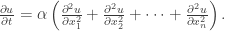
For convenience, we’ll denote the RHS operation $\sum_i \frac{\partial^2}{\partial x_i^2}$ by the symbol Δ or the “nabla-squared” symbol $\nabla^2$ . We’ll also call it the Laplacian operator. This gives an alternate way of writing the heat equation:

$\frac{\partial u}{\partial t} = \alpha \nabla^2 u \equiv \alpha \Delta u.$

Heat Kernel

The heat equation is usually given together with boundary conditions, e.g. the value of u(x, t) for t=0. This is completely analogous with our random walk, which starts with some probability distribution at t=0, then proceed at incremental discrete time steps. Another possibility is to start from t=0, and bound the system in space (e.g. x² + y² + z² ≤ r²) and specify the heat distribution at the space boundary as well (e.g. x² + y² + z² = r²).

Suppose, during t=0, the heat is all localised at the point x=0. This corresponds to the discrete case where our drunken friend starts at the point m=0. The function in this case is given by the Dirac delta function, δ(x), which unfortunately is not a function at all. Formally, δ(0)=”∞” and δ(x)=0 at x≠0, such that the integral ∫_R δ(x)dx = 1. This might seem baffling to mathematicians, but physicists have no qualms using it all the time. It’s possible to formally justify the δ(x) notation via the language of distributions, but that’s another story for another day.

Anyway, the solution (called the heat kernel) for this particular case is really nice. In the 1-D case, this is:

$u(x,t) = \frac 1 {\sqrt{4\pi \alpha t}} \exp(\frac{-x^2}{4\alpha t}).$

We’ll leave it to the reader to check that this equation satisfies the 1-D heat equation. Graphically, for α=1, this gives the plots:

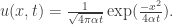
Notice that the probability distribution is a Gaussian (normal) curve which gradually spreads out as t increases. Also, the variance $\sigma^2 = 2\alpha t$ . This completely matches the discrete case of the drunken man (whose variance was 2pt)! The heat kernel also exists for the higher-dimensional case, but we need to replace x² by ∑_ix_i² in the formula for u.

In a nutshell, the heat kernel is the continuous variant of the probability distribution function for the drunken man problem.

However, there is an important distinction: for the discrete case the probability parameter cannot exceed 1/2, but for the PDE case, the parameter α can be any positive real number.

Independence of Coordinates

One important test to see if an equation makes “physical sense” is to check if it’s preserved under a change in coordinates. For example, vectors should be changed according to the coordinate transformation, while scalars should remain unchanged.

In n-dimensional space, transformation of a column vector corresponds to left multiplication by a fixed matrix A, i.e. $\mathbf{v} \mapsto A\mathbf{v}$ . Now dot-product of two column vectors can be written via the matrix notation $\mathbf{v}^t\mathbf{w}$ , since the transpose changes a column vector into a row. Thus, A preserves the inner product if and only if:

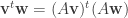
$\mathbf{v}^t\mathbf{w} = (A\mathbf{v})^t(A\mathbf{w})$

for all vectors v and w. Since (AB)^t = B^tA^t, the RHS simplifies to: $\mathbf{v}^t A^t A \mathbf{w}$ and the two sides are equal iff $A^t A = I$ .

Definition. An n × n real matrix A is said to be orthogonal if $A^t A = I$ . Via expanding this expression, one sees that A is orthogonal if and only if the column vectors are orthonormal.

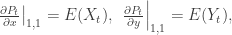
Now, let’s check that the heat equation is independent of our choice of coordinates. To do so, it suffices to check that the Laplacian operator $\Delta_x = \sum_i \frac{\partial^2}{\partial x_i^2}$ is coordinate-independent. The subscript x was added to highlight the fact that Δ was defined in terms of coordinate (x_i).

First, we write this operator as:

$\Delta_x = \frac{\partial^2}{\partial x_1^2} + \frac{\partial^2}{\partial x_2^2} + \ldots + \frac{\partial^2}{\partial x_n^2} = \nabla_x^t \nabla_x,$

where $\nabla_x$ is the column vector of differential operators comprising of $\frac{\partial}{\partial x_i}$ . [ This differential operator takes a scalar function f to the vector comprising of its partial derivatives. ]

Now suppose we have a different choice of coordinates which results in a transformation: $\mathbf{y} = A\mathbf{x}$ for some orthogonal matrix A. The corresponding transformation is given by:

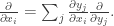
$\frac{\partial}{\partial x_i} = \sum_j \frac{\partial y_j}{\partial x_i} \frac{\partial}{\partial y_j}.$

Written in terms of the differential operator, we have: $\nabla_x = A\nabla_y$ . Now the Laplacian operator gives:

$\Delta_x = \nabla_x^t\cdot\nabla_x = (A\nabla_y)^t (A\nabla_y) = \nabla_y^t (A^tA)\nabla_y = \nabla_y^t \nabla_y = \Delta_y$

so the Laplacian is the same in both coordinates (x_i) and (y_i).

Conclusion. The heat equation is coordinate-independent, even though we had obtained it as a continuous variant of the drunken man problem which had explicitly chosen coordinates.

The above verification is non-trivial: e.g. if we had used the operator $\sum_i \frac{\partial}{\partial x_i}$ , the outcome would have been coordinate-dependent.

In higher physics, you’ll learn that one often obtains an equation simply because it’s the simplest one which “makes physical sense”, but that’d be another story for another day.

Posted in Notes | Tagged dirac delta function, heat equation, heat kernel, laplacian, orthogonal matrices, partial differential equations, random walk | Leave a comment

Random Walk and Differential Equations (I)

Posted on October 12, 2012 by limsup

Consider discrete points on the real line, indexed by the integers … -3, -2, -1, 0, 1, 2, … . A drunken man starts at position 0 and time 0. At each time step, he may move to the left or right (each with probability p<1/2), or stay still (with probability 1-2p).

This goes on and on, and we wish to find the probability distribution of his location at time t, i.e. for each m what’s the probability u(m, t) that he’s found at position m during time t? Clearly, for each t, $\sum_{m\in\mathbf{Z}} u(m,t) = 1$ since the man must be found somewhere.

To solve it exactly, one can use generating functions. Indeed, the recurrence relation in time gives:

$u(m, t+1) = p\cdot u(m-1, t) + p\cdot u(m+1, t) + (1-2p) u(m, t),$ (*)

for each integer m, non-negative integer t. So if we consider the power series

$P_t(x) = \ldots + u(-1, t)x^{-1} + u(0, t) + u(1, t)x + u(2,t)x^2 + \ldots = \sum_{m=-\infty}^\infty u(m,t)x^m,$

then the above recurrence relation in u(m, t) can be expressed succinctly as a recurrence relation in P_t(x):

$P_{t+1}(x) = (p\cdot x + p\cdot x^{-1} + (1-2p)) P_t(x),$

with $P_0(x) = 1$ . This expression has certain advantages in computation:

Example 1

Let x=1: this gives $P_{t+1}(1) = P_t(1)$ . But we already know this since P_t(1) represents the sum of all u(m, t) across m, i.e. it equals 1.

Example 2

Differentiate to obtain:

$P_{t+1}'(x) = (p - px^{-2})P_t(x) + (px + px^{-1} + (1-2p)) P_t'(x).$

Substitute x=1 to obtain $P_{t+1}'(1) = P_t'(1)$ . Since $P_0'(1) = 0$ , we also have $P_t'(1) = 0$ for all t. Again, we already know this since $P_t'(1) = \sum_m m\cdot u(m,t)$ represents the expected position of our friend, which is always 0 since he’s just as inclined to go left as he is to go right. In probability notation, we have $P_t'(1) = E(X_t)$ , where X_t is the random variable for our friend’s location at time t.

Example 3

Differentiate yet again to obtain:

$P_{t+1}''(x) = 2px^{-3} P_t(x) + 2(p-px^{-2})P_t'(x) + (px + px^{-1} + (1-2p))P_t''(x).$

Substitute x=1 to obtain $P_{t+1}"(1) = 2p P_t(1) + P_t''(1) = P_t''(1) + 2p$ . Since $P_0''(1) = 0$ we have $P_t''(1) = 2pt$ . But

$P_t''(x) = \sum_{m=-\infty}^\infty u(m,t)m(m-1)x^{m-2} \implies P_t''(1) = E(X_t(X_t-1)),$

so from $E(X_t) = 0$ we can calculate the variance via

$\text{Var}(X_t) = E(X_t^2) - E(X_t)^2 = 2pt.$

Example 4

Suppose the drunken man’s house is at x=5. What’s the value of $E((X_t - 5)^2)$ at time t?

Answer : let’s expand

$E((X_t - 5)^2) = E(X_t^2 - 10X_t + 25) = E(X_t^2) - 10 E(X_t) + 25 = 25 + 2pt$ .

Conclusion

As the reader can guess, successive differentiation gives us the higher moments $E(X_t^n)$ for various n. In fact, since

$P_{t+k}(x) = (p\cdot x + p\cdot x^{-1} + (1-2p))^k P_t(x),$

we can even consider relations across wider time steps.

Notice that we didn’t have to start with a fixed starting position for the drunken man. In particular, we could have any sequence of non-negative real u(m, 0), as long as the sum is 1. However, care would have to be taken to ensure that the higher moments are well-defined. E.g. if the probability distribution starts with

$u(m, 0) = \frac{6}{m^2\pi^2}$ for m>0 (u(m, 0) = 0 if m ≤ 0),

then the expected value is undefined since $\sum_{m=1}^\infty m\cdot u(m,0) = \frac{6}{\pi^2} \sum_{m=1}^\infty \frac 1 m$ which diverges since it is the renowned harmonic series. Roughly speaking, as m → ±∞, u(m, 0) should approach 0 exponentially fast in order for the higher moments to make sense.

Higher-Dimensional Case

Let’s assume now that our drunken friend can walk in a two-dimensional plane. So the probability of him at location (m, n) at time t is denoted u(m, n, t). At each time step, our friend can walk a unit distance in any of the four standard directions: north, south, east or west, each with probability p. The probability that he remains still for one time step is 1-4p.

The recurrence relation in t is easy to write:

u(m, n, t+1) = p(u(m-1, n, t) + u(m+1, n, t) + u(m, n-1, t) + u(m, n+1, t)) + (1-4p)u(m, n, t).

Proceeding as before, let’s define a two-parameter power series:

$P_t(x, y) = \sum_{m,n\in\mathbf{Z}} u(m,n,t) x^m y^n.$

The above recurrence relation then translates to:

$P_{t+1}(x,y) = (px + px^{-1} + py + py^{-1} +(1-4p))P_t(x,y).$

Let the random variable denoting his location at time t be (X_t, Y_t). In order to extract useful information, we’ll need to do partial differentiation. For convenience, we’ll denote $A(x,y) = px + px^{-1} + py + py^{-1} + (1-4p)$ .

$\frac{\partial P_{t+1}}{\partial x} = (p - px^{-2})P_t + A\cdot \frac{\partial P_t}{\partial x},$

$\frac{\partial P_{t+1}}{\partial y} = (p - py^{-2})P_t + A\cdot\frac{\partial P_t}{\partial y}.$

The second derivatives are:

$\frac{\partial^2 P_{t+1}}{\partial x^2} = 2px^{-3} P_t + 2(p - px^{-2})\frac{\partial P_t}{\partial x} + A\frac{\partial^2 P_t}{\partial x^2},$

$\frac{\partial^2 P_{t+1}}{\partial y^2} = 2py^{-3} P_t + 2(p - py^{-2})\frac{\partial P_t}{\partial x} + A\frac{\partial^2 P_t}{\partial y^2},$

$\frac{\partial^2 P_{t+1}}{\partial x\partial y} = (p-py^{-2})\frac{\partial P_t}{\partial x} + (p-px^{-2})\frac{\partial P_t}{\partial y} + A\frac{\partial^2 P_t}{\partial x\partial y}.$

Substituting x=1, y=1 gives the following useful values:

$\left.\frac{\partial P_t}{\partial x}\right|_{1,1} = E(X_t), \ \left.\frac{\partial P_t}{\partial y}\right|_{1,1} = E(Y_t),$

$\left.\frac{\partial^2 P_t}{\partial x^2}\right|_{1,1} = E(X_t^2 - X_t),\ \left.\frac{\partial^2 P_t}{\partial y^2}\right|_{1,1} = E(Y_t^2 - Y_t),\ \left.\frac{\partial^2 P_t}{\partial x\partial y}\right|_{1,1} = E(X_t Y_t).$

In the next article, we’ll consider the limiting case, where the space and time intervals approach zero, and look at the corresponding differential equations.

Posted in Notes | Tagged generating functions, heat equation, partial differential equations, random walk | Leave a comment

Intermediate Group Theory (6)

Posted on October 10, 2012 by limsup

In this post, we’ll only focus on additive abelian groups. By additive, we mean the underlying group operation is denoted by +. The identity and inverse of x are denoted by 0 and –x respectively. Similarly, 2x+3y refers to x+x+y+y+y. Etc etc.

Let G be an abelian group and S a subset of G. Consider <S>: the subgroup generated by S. As we saw earlier, this comprises of all “words” in S, i.e. 0, a, b, c, a+b, 2a+c, a–b+a, …, where a, b, c, … are elements of S. But since G is now abelian, we can write each term in the form: $m_1 a_1 + m_2 a_2 + \ldots + m_n a_n$ , where each m_i is an integer and a_i‘s are distinct terms belonging to S. Thus:

$\left<S\right> = \{m_1 a_1 + m_2 a_2 + \ldots + m_n a_n : m_i\in \mathbf{Z}, a_i\in S\}$ .

Important note. There are always finitely many terms in the sum, although if S is infinite, there is no upper bound to the number of terms. If S is finite, clearly the number of terms is upper-bounded by #S.

Summary. If G is abelian, then <S> is easily described as the set of all finite Z-linear combinations of elements of S.

Free Abelian Groups

Just like the case of free groups, we now consider an arbitrary set S and consider the set of all formal Z-linear combinations of S. By this, we mean the set of all symbolic expressions of finite-length as follows:

$F_{ab}(S)=\{ m_1 a_1 + m_2 a_2 + \ldots + m_n a_n : m_i\in\mathbf{Z}, a_i\in S\},$

with the understanding that the expression is unchanged if we add or remove terms of the form 0·x (x in S). Addition between elements of F_ab(S) is given term-wise, e.g. the sum of a+3b-2c and b+2c–d is a+4b–d. The resulting group F_ab(S) is called the free abelian group generated by S.

Universal Property.

The free abelian group satisfies a similar universal property: let i : S → F_ab(S) be the map which takes x to 1·x. Then for any function f : S → G to an abelian group G, there exists a unique group homomorphism g : F_ab(S) → G such that gi = f.

The map g itself is easy to describe: it takes the formal sum $m_1 a_1 + \ldots + m_n a_n$ (where $m_i\in \mathbf{Z}, a_i\in S$ ) to the element $m_1 f(a_1) + \ldots + m_n f(a_n)$ .

Direct Sums and Direct Products

Here is when things get a little more abstract. Consider a collection of abelian groups H_i, where i runs through a (possibly infinite) index set I. We’ll construct two groups: the direct sum and the direct product.

Definition. The direct product of the H_i‘s is the set:

$G = \prod_{i\in I} H_i = \{(x_i)_{i\in I} :x_i\in H_i\}$

where the group operation is given by component-wise product, i.e. $(x_i) + (y_i) = (x_i + y_i) \in \prod H_i$ . The direct sum is the subgroup:

$G' = \oplus_{i\in I} H_i =\{(x_i) \in \prod H_i : x_i \ne 0 \text{ for only finitely many } i\}.$

In short, the direct sum only contains those elements whose components are all 0 except possibly at finitely many places. For example, if we have I = {0, 1, 2, … } and each H_i = Z, then the direct product $\prod H_i$ is precisely the set of all integer sequences; while the direct sum $\oplus H_i$ is the set of all integer sequences with only finitely many non-zero entries.

In particular, for any set S, the free abelian group generated by S is the direct sum of (possibly infinitely many) copies of Z, indexed by S. In symbolic form,

$F_{ab}(S) = \oplus_{i\in S} \mathbf{Z}.$

No doubt the reader will ask: what’s the point of the two different definitions?

In order to explain that, we have to go into universal properties again. Basically, the two constructions satisfy two different types of universal properties. One can even say, after looking at the diagrams, that the two constructions are dual to each other.

More Universal Properties

First look at the direct product $G=\prod_i H_i$ . For every index i, there is a projection map $p_i : G \to H_i$ which takes (x_i)_i to the i-th component x_i. This gives us a whole bunch of maps p_i. The gist of the matter is as follows.

Universal Property 1. For any abelian group K, together with a collection of homomorphisms $q_i : K\to H_i$ , there is a unique homomorphism $f:K\to G=\prod_i H_i$ such that $p_i\circ f=q_i$ for every i.

In diagram form, we have:

How does the map f work? It takes an $x\in K$ to the element $(q_i(x))_{i\in I}$ which is an element of $\prod_i H_i$ . The fact that f is a homomorphism follows from the fact that all the q_i‘s are.

Now let’s look at the direct sum $G' = \oplus_i H_i$ . For each index i, we get an injection $e_i : H_i \to G'$ which takes $x_i \in H_i$ to the element (…, 0, 0, …, 0, x_i, 0, … ) in G’, i.e. all components are 0 except the i-th component, which takes the value of x_i.

Universal Property 2. For every abelian group K and a collection of group homomorphisms $f_i:H_i \to K$ , there is a unique homomorphism $g:\oplus_i H_i \to K$ such that $g\circ e_i = f_i$ for each i.

In diagram form, we now have:

Let’s define the map g. Each element of $\oplus_i H_i$ is a multi-component $(x_i)\in \prod_i H_i$ , where all but finitely many x_i‘s are zero. So we can let g take (x_i) to $\sum_i f_i(x_i)$ . This is a well-defined sum since there’re only finitely many non-zero terms (we don’t know how to sum infinitely many terms without some form of convergence).

Summary. We can describe the universal properties as follows. For direct product:

$\prod_{i\in I} \text{Hom}(K, H_i) \cong\text{Hom}(K, \prod_{i\in I} H_i).$

For direct sum:

$\prod_{i\in I} \text{Hom}(H_i, K) \cong\text{Hom}(\oplus_{i\in I}H_i, K).$

Exercises. Here’re some exercises to enhance your concepts of direct sum & direct product.

In the universal property diagram for direct product, replace $\prod_i H_i$ with $\oplus_i H_i$ instead. How does the universal property fail?
In the universal property diagram for direct sum, replace $\oplus_i H_i$ with $\prod_i H_i$ instead. How does the universal property fail?
Replace “abelian groups” and “homomorphisms” with “sets” and “functions” respectively. Explain what the corresponding direct sum and direct product are in this context, i.e. find appropriate constructions which satisfy the universal properties.
(Hard) Replace “abelian groups” with “groups”. Find the corresponding direct sum and direct product, i.e. find constructions which satisfy the universal properties. Note: the direct product is easy, but direct sum is much harder!

Hints for the Exercises. The following are ROT-13 encoded.

Fhccbfr k vf na ryrzrag bs X fhpu gung abar bs gur dv’f gnxr k gb gur vqragvgl. Gura s vf abg jryy-qrsvarq ba k. Va bgure jbeqf, s znl abg rkvfg.
Guvf vf nyernql rkcynvarq va gur grkg. Vs jr unir na ryrzrag bs gur qverpg cebqhpg, jubfr pbzcbaragf ner nyy aba-mreb, gura jr znl unir gb fhz npebff vasvavgryl znal aba-mreb ryrzragf. Fb t vf abg jryy-qrsvarq.
Gur qverpg fhz vf gur qvfwbvag havba bs gur frgf. Gur qverpg cebqhpg vf gur frg gurbergvp cebqhpg.
Gur qverpg cebqhpg vf vqragvpny gb gur pnfr sbe noryvna tebhcf. Gur qverpg fhz vf zhpu gevpxvre: vg pbzcevfrf bs “jbeqf” jubfr punenpgref ner ryrzragf bs vaqvivqhny tebhcf, jurer arvtuobhevat punenpgref orybat gb qvfgvapg tebhcf. Tebhc cebqhpg vf qrsvarq ol pbapngrangvat jbeqf gbtrgure, naq erzbivat erqhaqnapl vs gur ynfg punenpgre bs gur cerivbhf jbeq orybatf gb gur fnzr tebhc nf gur svefg punenpgre bs gur arkg jbeq.

Posted in Notes | Tagged abelian groups, advanced, direct products, direct sums, free groups, generated groups, universal properties | Leave a comment

Mathematics and Such

Introduction to Ring Theory (5)

Case of Commutative Rings

Chinese Remainder Theorem

Introduction to Ring Theory (4)

First Isomorphism Theorem

Second + Third Isomorphism Theorems

Introduction to Ring Theory (3)

Ideals and Ring Quotients

Operations on Ideals

Generated Ideals

Introduction to Ring Theory (2)

Subrings

Generated Subrings

Introduction to Ring Theory (1)

Examples

Intuition

Random Walk and Differential Equations (II)

1-Dimensional Heat Equation

Higher Dimensional Heat Equation

Heat Kernel

Independence of Coordinates

Random Walk and Differential Equations (I)

Higher-Dimensional Case

Intermediate Group Theory (6)

Free Abelian Groups

Direct Sums and Direct Products

More Universal Properties

Recent Posts

Archives

Categories

Meta

Pages