Random Walk and Differential Equations (II)

1-Dimensional Heat Equation

Consider the case of 1-dimensional random walk. The equation (*) from the previous post gives:

$u(x, t+1) = p\cdot u(x-1, t) + p\cdot u(x+1, t) + (1-2p) u(x, t),$

for t≥0. Suppose the intervals between successive time/space points are variable. Let’s rewrite it in the following form:

$\begin{aligned} u(x, t+\delta t) &= p\cdot u(x-\delta x, t) + p\cdot u(x+\delta x, t) + (1-2p)u(x,t)\\ \implies u(x, t+\delta t) - u(x,t) &= p(u(x+\delta x, t) - 2u(x, t) + u(x-\delta x, t)).\end{aligned}$

Setting δt ≈ ε² and δx ≈ ε, we divide both sides by ε² to obtain:

$\frac{\partial u}{\partial t} \approx \frac{u(x, t+\delta t) - u(x,t)}{\delta t} = p\frac{u(x+\delta x, t) - 2u(x,t) + u(x-\delta x, t)}{(\delta x)^2}.$ (#)

From the approximation,

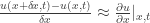
$\frac{u(x+\delta x, t)-u(x,t)}{\delta x} \approx \frac{\partial u}{\partial x}|_{x,t}$ ,

we see that the RHS of (#) approximates with $p\frac{\partial^2 u}{\partial x^2}$ .

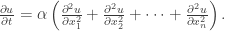
Definition. The 1-dimensional heat equation is the following partial differential equation (for some parameter α):

$\frac{\partial u}{\partial t} = \alpha\frac{\partial^2 u}{\partial x^2}$ .

This makes sense if we consider the kinetic theory of particles. Assume that we have a bunch of particles placed at equal intervals along a line. Heat of a particle refers to the amount of energy it possesses. At each time interval, the heat may transmit to a neighbouring particle (either to the left or right) or it may remain with the current particle. Since u(x, t) plots the amount of heat at each spacetime point, the random walk model is a reasonable approximation, whose limit gives us the heat equation.

Higher Dimensional Heat Equation

Let’s consider the two-dimensional case. We get the recurrence relation in time:

u(x, y, t+1) = p(u(x-1, y, t) + u(x+1, y, t) + u(x, y-1, t) + u(x, y+1, t)) + (1-4p)u(x, y, t).

Let’s re-express the above as follows, using arbitrary space and time interval lengths:

$\begin{array}{rl}u(x, y, t+\delta t) - u(x,y,t) &= p[u(x+\delta x,y,t)-2u(x,y,t)+u(x-\delta x,y,t)]\\ &+p[u(x,y+\delta y,t) - 2u(x,y,t) + u(x,y-\delta y,t)]\end{array}$

As before, if we set δt ≈ ε² and δx = δy ≈ ε then divide both sides by ε², we get:

LHS $\approx\frac{\partial u}{\partial t}$ ;
RHS $\approx p\left(\frac{\partial^2 u}{\partial x^2} + \frac{\partial^2 u}{\partial y^2}\right)$ .

Thus, let’s define the higher-dimensional heat equation as follows: if we have orthogonal coordinates x₁, x₂, …, x_n, then the n-dimensional heat equation is given by (for some parameter α):

$\frac{\partial u}{\partial t} = \alpha \left(\frac{\partial^2 u}{\partial x_1^2} + \frac{\partial^2 u}{\partial x_2^2} + \dots + \frac{\partial^2 u}{\partial x_n^2}\right).$

For convenience, we’ll denote the RHS operation $\sum_i \frac{\partial^2}{\partial x_i^2}$ by the symbol Δ or the “nabla-squared” symbol $\nabla^2$ . We’ll also call it the Laplacian operator. This gives an alternate way of writing the heat equation:

$\frac{\partial u}{\partial t} = \alpha \nabla^2 u \equiv \alpha \Delta u.$

Heat Kernel

The heat equation is usually given together with boundary conditions, e.g. the value of u(x, t) for t=0. This is completely analogous with our random walk, which starts with some probability distribution at t=0, then proceed at incremental discrete time steps. Another possibility is to start from t=0, and bound the system in space (e.g. x² + y² + z² ≤ r²) and specify the heat distribution at the space boundary as well (e.g. x² + y² + z² = r²).

Suppose, during t=0, the heat is all localised at the point x=0. This corresponds to the discrete case where our drunken friend starts at the point m=0. The function in this case is given by the Dirac delta function, δ(x), which unfortunately is not a function at all. Formally, δ(0)=”∞” and δ(x)=0 at x≠0, such that the integral ∫_R δ(x)dx = 1. This might seem baffling to mathematicians, but physicists have no qualms using it all the time. It’s possible to formally justify the δ(x) notation via the language of distributions, but that’s another story for another day.

Anyway, the solution (called the heat kernel) for this particular case is really nice. In the 1-D case, this is:

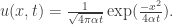
$u(x,t) = \frac 1 {\sqrt{4\pi \alpha t}} \exp(\frac{-x^2}{4\alpha t}).$

We’ll leave it to the reader to check that this equation satisfies the 1-D heat equation. Graphically, for α=1, this gives the plots:

Notice that the probability distribution is a Gaussian (normal) curve which gradually spreads out as t increases. Also, the variance $\sigma^2 = 2\alpha t$ . This completely matches the discrete case of the drunken man (whose variance was 2pt)! The heat kernel also exists for the higher-dimensional case, but we need to replace x² by ∑_ix_i² in the formula for u.

In a nutshell, the heat kernel is the continuous variant of the probability distribution function for the drunken man problem.

However, there is an important distinction: for the discrete case the probability parameter cannot exceed 1/2, but for the PDE case, the parameter α can be any positive real number.

Independence of Coordinates

One important test to see if an equation makes “physical sense” is to check if it’s preserved under a change in coordinates. For example, vectors should be changed according to the coordinate transformation, while scalars should remain unchanged.

In n-dimensional space, transformation of a column vector corresponds to left multiplication by a fixed matrix A, i.e. $\mathbf{v} \mapsto A\mathbf{v}$ . Now dot-product of two column vectors can be written via the matrix notation $\mathbf{v}^t\mathbf{w}$ , since the transpose changes a column vector into a row. Thus, A preserves the inner product if and only if:

$\mathbf{v}^t\mathbf{w} = (A\mathbf{v})^t(A\mathbf{w})$

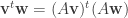
for all vectors v and w. Since (AB)^t = B^tA^t, the RHS simplifies to: $\mathbf{v}^t A^t A \mathbf{w}$ and the two sides are equal iff $A^t A = I$ .

Definition. An n × n real matrix A is said to be orthogonal if $A^t A = I$ . Via expanding this expression, one sees that A is orthogonal if and only if the column vectors are orthonormal.

Now, let’s check that the heat equation is independent of our choice of coordinates. To do so, it suffices to check that the Laplacian operator $\Delta_x = \sum_i \frac{\partial^2}{\partial x_i^2}$ is coordinate-independent. The subscript x was added to highlight the fact that Δ was defined in terms of coordinate (x_i).

First, we write this operator as:

$\Delta_x = \frac{\partial^2}{\partial x_1^2} + \frac{\partial^2}{\partial x_2^2} + \ldots + \frac{\partial^2}{\partial x_n^2} = \nabla_x^t \nabla_x,$

where $\nabla_x$ is the column vector of differential operators comprising of $\frac{\partial}{\partial x_i}$ . [ This differential operator takes a scalar function f to the vector comprising of its partial derivatives. ]

Now suppose we have a different choice of coordinates which results in a transformation: $\mathbf{y} = A\mathbf{x}$ for some orthogonal matrix A. The corresponding transformation is given by:

$\frac{\partial}{\partial x_i} = \sum_j \frac{\partial y_j}{\partial x_i} \frac{\partial}{\partial y_j}.$

Written in terms of the differential operator, we have: $\nabla_x = A\nabla_y$ . Now the Laplacian operator gives:

$\Delta_x = \nabla_x^t\cdot\nabla_x = (A\nabla_y)^t (A\nabla_y) = \nabla_y^t (A^tA)\nabla_y = \nabla_y^t \nabla_y = \Delta_y$

so the Laplacian is the same in both coordinates (x_i) and (y_i).

Conclusion. The heat equation is coordinate-independent, even though we had obtained it as a continuous variant of the drunken man problem which had explicitly chosen coordinates.

The above verification is non-trivial: e.g. if we had used the operator $\sum_i \frac{\partial}{\partial x_i}$ , the outcome would have been coordinate-dependent.

In higher physics, you’ll learn that one often obtains an equation simply because it’s the simplest one which “makes physical sense”, but that’d be another story for another day.