Mathematics and Such

Basic Analysis: Limits and Continuity (2)

Posted on November 23, 2012 by limsup

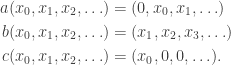
Previously, we defined continuous limits and proved some basic properties. Here, we’ll try to port over more results from the case of limits of sequences.

Monotone Convergence Theorem. If f(x) is increasing on the open interval (c, a) and has an upper bound, then $\lim_{x\to a^-} f(x)$ exists.

[ Recall that by “increasing”, we mean: if x ≤ y, then f(x) ≤ f(y). In particular, even a constant function is considered “increasing” under our definition. ]

Proof.

As before let L = sup{f(x) : c < x < a}, which is finite since f(x) has an upper bound. For each ε>0, since L-ε is not an upper bound, there exists δ>0 such that L-ε < f(a-δ) ≤ L. Hence, for any a-δ < x < a, we also have f(x) ≥ f(a-δ) > L-ε and f(a-δ) ≤ L. ♦

Note that this theorem has many variations. For example, f(x) can be either monotonically increasing or decreasing. Or the limit can be either left or right. Here’re two possibilities:

If f(x) is decreasing on (a, b) and has an upper bound, then $\lim_{x\to a^+} f(x)$ exists.
If f(x) is increasing on (-∞, b) and has a lower bound, then $\lim_{x\to -\infty} f(x)$ exists.

Example

Define 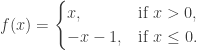$f(x) =\begin{cases} x, &\text{if } x>0, \\ -x-1, &\text{if } x\le 0.\end{cases}$ Now f is an increasing function and is bounded on (-1, 1) so the left and right limits $\lim_{x\to 0^-} f(x)$ , $\lim_{x\to 0^+} f(x)$ both exist. However, the left limit is -1 while the right limit is 0. Since both limits are not equal, $\lim_{x\to 0} f(x)$ does not exist even though f is monotone and bounded.

Next, we have the following.

Squeeze Theorem. Suppose $g(x) \le f(x) \le h(x)$ on the open interval (c, a). If

$\lim_{x\to a^-} g(x) = \lim_{x\to a^-} h(x) = L,$

then $\lim_{x\to a^-} f(x) = L$ as well. This holds for the limits $\lim_{x\to a^+}$ and $\lim_{x\to a}$ as well.

Proof.

We’ll only prove the case for left limits. Let ε>0. Then there exist positive δ₁ and δ₂ such that:

whenever a-δ₁ < x < a, we have |g(x) – L| < ε;
whenever a-δ₂ < x < a, we have |h(x) – L| < ε.

Hence if δ = min(δ₁, δ₂), then whenever a-δ < x < a, we have f(x) ≤ h(x) < L+ε and f(x) ≥ g(x) > L-ε. Thus |f(x) – L| < ε. ♦

Example

Consider the function $f(x) = x \sin(1/x)$ , for x≠0. Then:

$-|x|\le f(x) \le |x|$ , for all x≠0.

Since $\lim_{x\to 0} |x| = \lim_{x\to 0} (-|x|) = 0$ , it follows from the Squeeze Theorem that $\lim_{x\to 0} f(x) = 0$ .

(Graphs plotted by wolframalpha.com)

Continuous Functions: Basic Concepts

We wish to define what it means for a function to be continuous at x=a. It’s natural to define it in terms of limits.

Definition. Suppose f(x) is defined on an open interval (b, c) containing a. We say that f is continuous at a, if

$\lim_{x\to a} f(x) = f(a)$ .

Equivalently, we say that f is continuous at a, if for every ε>0, there exists δ>0, such that:

$|x-a|<\delta \implies |f(x)-f(a)|<\epsilon.$

Example

For example, let’s consider $f(x) = \begin{cases} x\sin(1/x), &\text{if }x\ne 0, \\ 0, &\text{otherwise}.\end{cases}$ .

Since $\lim_{x\to 0} f(x) = 0 = f(0)$ , we see that f is continuous at x=0. ♦

The second definition is really neat, because now even if f(x) is not defined on an open interval about a, we can talk about continuity at a itself. To be explicit, suppose D is a subset of the reals R, and f : D → R is a function. If a lies in D, we say that f(x) is continuous at x=a if:

for every ε>0, there exists δ>0, such that whenever |x–a|<δ and x lies in D, we have |f(x)-f(a)|<ε.

Example

Consider the function $f(x) = \begin{cases} x, &\text{if } x> 1, \\ 0.5, &\text{if }x=0, \\ -x, &\text{if } x< -1.\end{cases}$ , which is defined on $D = (-\infty, -1)\cup\{0\}\cup(+1,\infty)$ .

Strange as it may sound, f(x) is continuous at x=0 according to our definition. Indeed, let’s check the definition. When someone throws an ε>0 at us, we have to produce a δ>0, such that if |x-0| = |x| < δ and x lies in D, then |f(x)-f(0)| = |f(x)-0.5| < ε. What can this δ be? It’s clear that δ=0.5 works for any ε(!), for the condition “|x| < 0.5 and x lies in D” is satisfied by one and only one point: namely, x=0, in which case |f(x)-f(0)|=0.

It’s also clear from the proof that we’re at complete liberty to shift f(0) to any point we wish and the function is still continuous. This occurs due to an anomaly in the domain of definition D. As the point x=0 is too far from its neighbours, f(0) can take whatever the heck it wants without breaking continuity.

So when is f(a) uniquely determined by continuity?

Definition. Let D be a subset of R. A real number a is called a point of accumulation (or cluster point, or limit point) if for every ε>0, there exists $x\in D, x\ne a$ such that |x-a|<ε.

In short a is a point of accumulation if there are points of D which are arbitrarily close to it. E.g. in the above example $D = (-\infty,-1)\cup\{0\}\cup(1,\infty)$ , the point 0 is not a point of accumulation. On the other hand, -1 and +1 are points of accumulation even though they don’t lie in D. As a final example, for the set {1, 1/2, 1/3, … }, 0 is a point of accumulation.

The result we wish to prove is the following.

Definition. Let D be a subset of R and a be point of accumulation of D. If two functions

$f, g:D\cup\{a\} \to \mathbf{R}$

agree on D-{a} and are continuous at a, then f(a) = g(a).

Proof.

If not, let ε = |f(a)-g(a)|/2. Then there exist positive δ₁ and δ₂ such that:

$|x-a|<\delta_1 \implies |f(x)-f(a)|<\epsilon$ ;
$|x-a|<\delta_2 \implies |g(x)-g(a)|<\epsilon$ .

Since a is a point of accumulation, we can pick an x in D such that 0 < |x–a| < min(δ₁, δ₂). This x satisfies f(x)=g(x) by condition, thus giving:

which is absurd. ♦

Further Properties

As the reader may suspect, we also have the following properties: if $f, g :D\to \mathbf{R}$ are both continuous at a, then

f+g : D → R is continuous at a;
fg : D → R is continuous at a;
if f(a)≠0, then 1/f : D’ → R is continuous at a, where D’ is the set of x in D for which f(x)≠0.

The proof is extremely similar to the case of limits, so we’ll skip it for now. The conscientious reader may want to prove the above results to convince himself/herself, but we’ll prove them as a corollary in the next article by looking at higher-dimensional continuity.

As a consequence, since constant functions f(x)=c and the identity function f(x)=x are both continuous at every point in R, so is any polynomial function.

Exercises

Prove that if a is not a point of accumulation of D, then any function $f:D\cup\{a\} \to\mathbf{R}$ is automatically continuous at a.
Prove that if f : (c, a] → R is a function, where (c, a] is the set of x, c < x ≤ a, then f is continuous at a if and only if $\lim_{x\to a^-} f(x) = f(a)$ .
Let f : D → R be a function. Prove that f(x) is continuous at a if and only if for every sequence (x_n) in D which converges to a, the sequence f(x_n) also converges to f(a).

Posted in Notes | Tagged advanced, analysis, continuity, limits, monotone convergence theorem, points of accumulation, squeeze theorem | Leave a comment

Basic Analysis: Limits and Continuity (1)

Posted on November 20, 2012 by limsup

[ This is a continuation of the series on Basic Analysis: Sequence Convergence. ]

In this article, we’ll describe rigourously what it means to say things like $\lim_{x\to 3} f(x) = 6$ . First, we define a punctured neighbourhood of a real number a to be a set of the form: (a-ε, a+ε) – {a}, i.e. the set $\{x\in\mathbf{R} : 0<|x-a|<\epsilon\}$ for some positive ε.

For example, here’s a punctured neighbourhood of 3:

Definition. Suppose f(x) is a function defined on a punctured neighbourhood of a real number a. We write $\lim_{x\to a} f(x) = L$ if:

for any real ε>0, there is a real δ>0, such that if x is a real number satisfying 0<|x-a|<δ, we have |f(x)-L|<ε.

Pictorially, we have:

Example 0.

The limit is unique, i.e. if $\lim_{x\to a} f(x) = K$ and $\lim_{x\to a} f(x) = L$ , then K=L.

Proof.

If K ≠ L, let ε = |K–L|/2. By definition of limits,

there exists δ such that for all x satisfying 0 < |x–a| < δ, we have |f(x)-K| < ε;
there exists δ’ such that for all x satisfying 0 < |x–a| < δ’, we have |f(x)-L| < ε.

Picking x such that 0 < |x–a| < min(δ, δ’), we find that both conditions are satisfied, so

$|K-L| \le |K-f(x)| + |f(x)-L| < 2\epsilon = |K-L|$ ,

clearly a contradiction. ♦

Example 1.

Let $f(x) = \frac{x^2 - 5x + 6}{x-2}$ , defined on x≠2. Prove that $\lim_{x\to 2} f(x) = -1$ .

Proof.

When x≠2, we have f(x) = (x-2)(x-3)/(x-2) = x-3. Hence, for each ε, just pick δ=ε. Now, whenever 0<|x-2|<δ=ε, we have |f(x)+1| = |x-2| < ε. By definition this means $\lim_{x\to 2}f(x) = -1$ . ♦

Example 2.

Let f(x) = sgn(x), defined on x≠0, which takes x to +1 if x>0 and -1 if x<0. Prove that $\lim_{x\to 0}f(x)$ does not exist.

Proof.

Again we need to negate the definition of limits: to show that for every L, there exists an ε>0, such that for every δ>0, we can find x satisfying 0<|x|<δ but |f(x)-L| ≥ ε. [ Reason this out carefully if it’s not clear. ]

Indeed, regardless of L, pick ε=1/2. Now given any δ>0, we can pick

x = +δ/2 : this gives 0<|x|<δ, but f(x)=+1;
y = -δ/2 : this gives 0<|y|<δ, but f(y)=-1.

We claim that |f(x)-L| ≥ ε or |f(y)-L| ≥ ε. If not, both |f(x)-L| and |f(y)-L| are less than ε,

$2 = |f(x) - f(y)| \le |f(x)-L| + |L-f(y)| < \epsilon+\epsilon = 1$

which is absurd. Hence, f(x) does not approach L as x→0, regardless of what L is. ♦

Properties of Limits

We have the following properties, which are similar to the case for the limit of a sequence.

Theorem. Let f(x), g(x) be functions defined on a punctured neighbourhood of a. Suppose $\lim_{x\to a}f(x) = K$ and $\lim_{x\to a}g(x)=L$ . Then:

$\lim_{x\to a} (f(x)+g(x)) = K+L$ ;

for some δ>0, B>0, we have $0<|x-a|<\delta\implies |f(x)|<B$ ;

$\lim_{x\to a} f(x)g(x) = KL$ ;

if L≠0, then $\lim_{x\to a} 1/g(x) = 1/L$ .

Note.

Property 2 differs from the case of a converging sequence, which is always bounded. Back then, we only needed to exclude finitely many terms of a sequence which lie outside a “safe zone”; here, we always have infinitely many points outside a “safe interval”.

In the remaining of this article, we’ll use the mnemonic “P(x) holds when x is close to a“, to mean “there exists δ>0, such that whenever 0<|x-a|<δ, P(x) holds“. Now, the definition of continuous limit can be shortened to:

for each ε>0, |f(x)-L|<ε when x is close to a.

Once again, if the statements “P(x) holds when x is close to a” and “Q(x) holds when x is close to a” are both true, then we can also confidently declare “(P(x) and Q(x)) hold when x is close to a“. In particular, we can repeat this finitely many times and concatenate finitely many properties together. Just don’t do this for infinitely many statements.

Now we’re ready to prove the above properties.

Proof.

For the first property, let ε>0. By definition of limits, we have |f(x)-K| < ε/2 when x is close to a, and |g(x)-L| < ε/2 when x is close to a. Thus, |f(x)-K| < ε/2 and |g(x)-L| < ε/2 both hold when x is close to a, which gives us

$|f(x)+g(x)-(K+L)| \le |f(x)-K|+|g(x)-L| < \frac\epsilon 2 + \frac\epsilon 2 =\epsilon.$

The second property says there exists B>0 such that |f(x)|<B for x close to a. This follows straight from the definition.

For the third property, write:

$|f(x)g(x)-KL| = |(f(x)-K)g(x) + K(g(x)-L)| \le |f(x)-K|\cdot |g(x)| + |K|\cdot |g(x)-L|.$

Let ε>0. Now we have:

by the second property, there is a bound B such that |g(x)|<B for x close to a;
by definition of limit, |f(x)-K| < ε/(2B) for x close to a;
again by definition of limit, |g(x)-L| < ε/(2L) for x close to a.

Putting it all together, |f(x)g(x) – KL| < ε for x close to a. We’ll leave the fourth property for the reader. ♦

As corollaries, we obtain:

$\lim_{x\to a} c\cdot f(x) = c\cdot K$ for any real c;
$\lim_{x\to a} (f(x)-g(x)) = K-L$ ;
$\lim_{x\to a} f(x)^n = K^n$ for n=1, 2, … ; if K≠0, this even holds for all integers n;
if L≠0, then $\lim_{x\to a} f(x)/g(x) = K/L$ .

To prove the first statement, apply property 3 with the constant function g(x)=c. For the second statement, write f(x)-g(x) = f(x)+(-1)g(x). The third statement follows from properties 3 and 4 via successive multiplication/division. For the final statement, write f(x)/g(x) = f(x) × (1/g(x)) and apply properties 3 and 4 above.

Example 3.

Prove that if $f(x) = \frac{x^2 + 4x + 5}{x^3 + 1}$ , then $\lim_{x\to 1} f(x) = 5$ .

Proof.

Start from $\lim_{x\to 1} x = 1$ , which can be easily proven from ε-δ definition. Now, apply the above properties successively: $\lim_{x\to 1} x^2 = 1$ , $\lim_{x\to 1}(x^2 + 4x + 5) = 10$ … . ♦

More Limits

Often, we encounter functions which are only defined for x>a, in which case the limit approaches from only one side.

Definition. Let f(x) be defined on the open interval (a, b) for some b>a. We write $\lim_{x\to a^+} f(x) = L$ if:

for each ε>0, there exists a δ>0, such that whenever 0 < x-a < δ, we have |f(x)-L| < ε.

Likewise, suppose f(x) is defined on the open interval (c, a) for some c<a. We write $\lim_{x\to a^-} f(x)=L$ if:

for each ε>0, there exists a δ>0, such that whenever 0 > x-a > -δ, we have |f(x)-L| < ε.

Again, let’s use the mnemonics “P(x) holds when x is slightly more than a“, to mean there exists δ>0 such that P(x) holds for all 0 < x–a < δ. Likewise, “P(x) holds when x is slightly less than a” means there exists δ>0 such that P(x) holds for all 0 > x–a > -δ.

Example 4.

Suppose f(x) is defined on a punctured neighbourhood of a. Then:

if $\lim_{x\to a} f(x) = L$ , then $\lim_{x\to a^+} f(x) = \lim_{x\to a^-} f(x) = L$ ;
conversely, if $\lim_{x\to a^+} f(x) = \lim_{x\to a^-} f(x) = L$ (i.e. equal left and right limits), then $\lim_{x\to a} f(x) = L$ .

Sketch of Proof

This boils down to the fact that “P(x) holds for x close to a” is equivalent to saying that “P(x) holds for x slightly more than a” and “P(x) holds for x slightly less than a” are both true. We’ll leave it to the reader to fill in the details. ♦

Finally we’d also like to say $\lim_{x\to 0^+} 1/x = \infty$ , so there’s a need to talk about a limit “approaching infinity”. Then there’s the case where x itself can approach +∞ or -∞. All these cases multiply to a huge number of possibilities! We can summarise by saying:

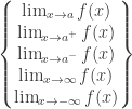$\left\{\begin{matrix} \lim_{x\to a} f(x)\\ \lim_{x\to a^+} f(x)\\ \lim_{x\to a^-} f(x)\\ \lim_{x\to\infty} f(x) \\ \lim_{x\to -\infty} f(x)\end{matrix}\right\}$ = $\left[\begin{matrix} L \\ \infty\\-\infty\end{matrix}\right]$ if for every $\left[\begin{matrix} \epsilon>0 \\ N \\ N\end{matrix}\right]$ there exists $\left\{\begin{matrix} \delta>0\\ \delta>0\\ \delta>0\\ M \\M\end{matrix}\right\}$ such that

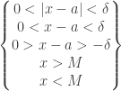whenever x satisfies $\left\{\begin{matrix} 0<|x-a|<\delta\\ 0<x-a<\delta \\ 0>x-a>-\delta\\ x>M\\ x<M\end{matrix}\right\}$ , we have $\left[\begin{matrix} |f(x)-L|<\epsilon\\ f(x)>N \\ f(x)<N\end{matrix}\right]$ .

Here, the square brackets match each other while the curly brackets also match. So all in all, we get 15 definitions in a single statement.

But the vast number of possibilities can overwhelm us when we try to prove even the simplest properties (imagine writing this article 15 times, with only minor differences across the articles). One wonders if there’s a better approach: the answer is yes, by considering topologies on the domain and codomain and thinking in general terms of limits, but that’s another story for another day. For now, we’ll just proceed as usual, focusing on one or two special cases for each result.

Posted in Notes | Tagged advanced, analysis, limits, punctured neighbourhoods | Leave a comment

Basic Analysis: Sequence Convergence (4)

Posted on November 17, 2012 by limsup

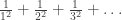
In this article, we’ll consider the convergence of an infinite sum: $a_1 + a_2 + a_3 + \ldots$ . We call this sum an infinite series. Let $s_n = a_1 + a_2 + \ldots + a_n$ be the partial sums of the series.

Definition. We say that $\sum_{n=1}^\infty a_i$ is L (resp. ∞, -∞) if the partial sums $(s_n)$ converge to L (resp. ∞, -∞). The series is said to be convergent if the sum is a real number L.

Example 1.

The series: $\frac 1{1\times 2} + \frac 1{2\times 3} + \frac 1{3\times 4} + \ldots$ converges to 1 since the partial sums

$\sum_{i=1}^n \frac 1{i(i+1)} = \sum_{i=1}^n \left(\frac 1 i-\frac 1{i+1}\right) = \left(1 - \frac 1 2\right) + \left(\frac 1 2 - \frac 1 3\right) + \ldots +\left(\frac 1 n-\frac 1 {n+1}\right)=1 - \frac 1{n+1}$

form a telescoping series. As n→∞, the RHS clearly converges to 1.

Example 2.

The series: $\frac 1 {1^2} + \frac 1 {2^2} + \frac 1{3^2} + \ldots$ converges. Indeed, we have $0 < \frac 1 {n^2} < \frac 1 {n(n-1)}$ , so upon dropping the first term (1), we can apply squeeze theorem on the partial sums to obtain:

$1 < \frac 1 {1^2} + \frac 1 {2^2} + \frac 1 {3^2} + \ldots < 1 + \frac 1 {1\times 2} + \frac 1 {2\times 3} + \ldots = 2.$

Computing the exact value is rather difficult and we won’t go into that now.

Example 3.

Consider the series $\sum_{n=1}^\infty \frac 1{4n^2-1}$ . We can write the sum in two different ways:

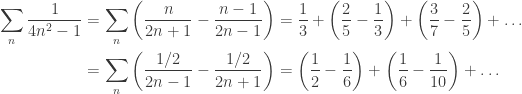
$\begin{aligned} \sum_n \frac 1{4n^2-1} &= \sum_n \left(\frac n{2n+1} -\frac {n-1}{2n-1}\right) =\frac 1 3 +\left(\frac 2 5 - \frac 1 3\right)+\left(\frac 3 7-\frac 2 5\right) + \ldots\\ &=\sum_n \left(\frac {1/2} {2n-1}-\frac{1/2}{2n+1}\right)= \left(\frac 1 2-\frac 1 6\right)+\left(\frac 1 6-\frac 1 {10}\right) + \ldots \end{aligned}$

All the terms in the first sum appear to cancel each other out, leaving a sum of zero, which is ridiculous since all the terms in the series are positive. However, a moment of thought reveals that the partial sums are really $\frac n{2n+1}$ which approaches 1/2. Hence, the series converges to 1/2, which is also obvious from the second sum.

Proposition. If the series $\sum a_n$ is convergent, then $(a_n) \to 0$ .

Proof.

Let ε>0. Since the partial sums converge to a real number, it is a Cauchy sequence so there exists N such that $|s_m - s_n| < \epsilon$ for all m, n > N. In particular, $|a_n| = |s_n-s_{n-1}| < \epsilon$ for all n > N+1. Hence, $(a_n) \to 0$ . ♦

Example 4.

The converse is not true: there’re many examples of sequences $(a_n)$ which converge to 0, but whose sums don’t converge. The most famous example is that of the harmonic series $1 + \frac 1 2 + \frac 1 3 + \ldots$ , where the sum of the first n terms is approximately log(n).

Basic Properties

Properties. Suppose $\sum_n a_n = L_1$ and $\sum_n b_n = L_2$ . Then:

$\sum_n (a_n + b_n) = L_1 + L_2$ ;

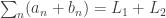$\sum_n (ca_n) = cL_1$ for any real c.

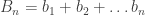Since the partial sums of (a_n + b_n) is the sum of the partial sum of a_n and that of b_n, the first property follows easily. Similarly, the second property follows from the fact that the partial sums of (c·a_n) are just c·(partial sums of a_n).

On the other hand, the sum of products ∑(a_nb_n) is quite a pain. One way of handling it is to use Abel transformation: write $B_n = b_1 + b_2 + \ldots b_n$ for the partial sums of b_n, then:

$\begin{aligned}\sum_{n=1}^m a_n b_n &= \sum_{n=1}^m a_n(B_n - B_{n-1}) = \sum_{n=1}^m a_n B_n - \sum_{n=0}^{m-1} a_{n+1} B_n= \sum_{n=1}^m B_n(a_n - a_{n+1})+ a_m B_m.\end{aligned}$

Example 5.

Prove that if the partial sums $s_n = a_1 + a_2 + \ldots + a_n$ are bounded, then $\frac{a_1}1 + \frac{a_2} 2 + \frac{a_3} 3 + \ldots$ converges.

Proof.

Let b_n = 1/n. By Abel transformation with a‘s and b‘s swapped, we get:

$\begin{aligned}\sum_{n=1}^m \frac{a_n} n = \sum_{n=1}^m s_n(b_n - b_{n+1}) + b_m s_m = -\sum_{n=1}^m \frac{s_n}{n(n+1)} + \frac{s_m}m.\end{aligned}$

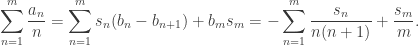
Since $(s_n)$ is bounded, the second term $\frac{s_m}m \to 0$ . Hence it suffices to show that $\sum_n \frac {s_n}{n(n+1)}$ converges. But since |s_n|≤L are bounded, we have:

$\begin{aligned}\left|\sum_{n=j}^k \frac{s_n}{n(n+1)}\right| \le \sum_{n=j}^k \frac{|s_n|}{n(n+1)} \le L\sum_{n=j}^k \frac 1{n(n+1)}.\end{aligned}$

Since $\sum_n \frac 1 {n(n+1)}$ converges, its partial sums form a Cauchy sequence. This in turn implies that the partial sums of $\sum_n \frac{s_n}{n(n+1)}$ form a Cauchy sequence, and we’re done. ♦

Theorem (Alternating Series Test). If $(a_n)$ is a decreasing sequence of positive values converging to 0, then the series $\sum_n (-1)^n a_n$ is convergent.

Proof.

Let b_n = (-1)ⁿ. Apply the Abel transformation:

$\begin{aligned}\sum_{n=1}^m a_n b_n =\sum_{n=1}^m B_n(a_n - a_{n+1})+ a_m B_m,\end{aligned}$

where $B_n = b_1 + \ldots + b_n$ and thus |B_n| ≤ 2. Since $a_m \to 0$ , we also have $a_m B_m \to 0$ so it suffices to show that $\sum_n B_n(a_n-a_{n+1})$ converges. Now,

$|\sum_{n=j}^k B_n(a_n - a_{n+1})| \overbrace{\le\sum_{n=j}^k |B_n|(a_n-a_{n+1})}^{\because (a_n) \text{ dec.}} \le 2(a_j-a_{k+1}).$

Since $(a_n)$ is convergent, it is also Cauchy, so the partial sums of $\sum_n B_n(a_n-a_{n+1})$ form a Cauchy sequence, and the series is convergent. ♦

Example 6.

Consider the infinite series $1 -\frac 1 2 + \frac 1 3 - \frac 1 4 + \ldots$ . By the alternating series test, the series converges, though the test doesn’t give any hint what the sum might be.

Permutation of a Series

If $\sum_{n\ge 1} a_n$ is a series, then we can permute the terms to obtain $\sum_{n\ge 1} a_{\pi(n)}$ , where π:N → N is a bijective function. For example:

we can switch the first two terms to obtain $a_2 + a_1 + a_3 + a_4 + \ldots$ , i.e. π(1) = 2, π(2) = 1, and π(m) = m for all m > 2;
we can switch each 2k-1 with 2k to obtain $a_2 + a_1 + a_4 + a_3 + a_6 + a_5 + \ldots$ , i.e. π(2k-1) = 2k, π(2k) = 2k-1 for k=1, 2, 3, … .

It may surprise the reader that the sum of an infinite series may depend on the order of summation, despite the fact that addition is commutative.

Example 7.

We already saw that $S =1 - \frac 1 2 + \frac 1 3 - \ldots$ is convergent. On the one hand, we can write:

$S = 1 - \left(\frac 1 2 - \frac 1 3\right) - \left(\frac 1 4 - \frac 1 5\right) -\ldots$

where each bracketed term is positive, so S < 1. On the other hand, let’s write S = 1 + sum of terms of the form:

$a_k = \frac 1 {4k-1} + \frac 1 {4k+1} -\frac 1 {2k} = \frac {8k}{16k^2-1} - \frac 1{2k} >0$ , k = 1, 2, 3, … .

This would imply that S > 1, so the sum of an infinite series can be changed by permuting the terms.

For a series to be better-behaved, we need the following concept:

Definition. The series $\sum_n a_n$ is said to converge absolutely if the series $\sum_n |a_n|$ converges. If $\sum a_n$ converges but not absolutely, we say it is conditionally convergent.

For example, the alternating series $1 - \frac 1 2 + \frac 1 3 - \ldots$ we saw above is only conditionally convergent. On the other hand, the alternating series $1 - \frac 1{2^2} + \frac 1 {3^2}-\ldots$ is absolutely convergent.

The key property we want to state is:

Theorem. If $\sum a_n$ converges absolutely, then every permutation of the series converges, and to the same sum.

Proof.

Let ε>0. Since the partial sums Σ|a_n| form a Cauchy sequence, for some N,

$|a_m| + |a_{m+1}| + \ldots + |a_n|< \epsilon/2$ for all n > m > N.

This immediately implies that the partial sums Σa_n form a Cauchy sequence and converges to some L. Now for any permutation π of {1, 2, 3, … }, we need to show that $\sum (a_{\pi(n)} - a_n) = 0$ . To do that, let:

$M = \max\{\pi^{-1}(1), \pi^{-1}(2), \ldots, \pi^{-1}(N)\}.$

Basically, the crux is that when n > M, π(n) > N. So when n > m > M, we have

$\begin{aligned}|\sum_{i=m}^n a_{\pi(i)} - a_i| \le \sum_{i=m}^n |a_{\pi(i)} - a_i| \le \sum_{i=m}^n (|a_{\pi(i)}| + |a_i|) <\frac\epsilon 2 + \frac\epsilon 2.\end{aligned}$

So $\sum (a_{\pi(n)} - a_n) \to 0$ as required. ♦

Hence, absolute convergence of a series ensures well behaviour. This fact carries on over to the “continuous case” where we can exchange integrating variables dx dy and dy dx if the absolute value of the integrand integrates to a finite real value. But that’s another story for another day.

Exercise.

Prove that if $\sum_n a_n$ is conditionally convergent, then for every real L, there is a permutation π of {1, 2, 3, … } such that $\sum_n a_{\pi(n)} = L$ .

[ Hint (highlight to read): let b_n and c_n be the positive and negative terms in the series (a_n) respectively. Show that Σb_n = ∞ and Σc_n = -∞. Now given L, pick just enough terms from b_n so that the sum exceeds L. Then pick just enough terms from c_n so that the sum drops below L. And so on. Show that b_n → 0 and c_n → 0 which implies the process eventually tends to L. ]

Posted in Notes | Tagged abel transformation, alternating series, analysis, basel series, convergence, series, telescoping series | Leave a comment

Basic Analysis: Sequence Convergence (3)

Posted on November 14, 2012 by limsup

So far, we’ve been considering the case where a sequence converges to a real number L. It’s also possible for a sequence to approach +∞ or -∞. The infinity symbol “∞” should be thought of as a convenient symbol instead of an actual infinity; in particular, it bears no relation to the cardinality (i.e. size) of the set of integers.

Definition. Let (a_n) be a sequence of real numbers. We write (a_n) → ∞ if

for every real M, there exists N such that if n>N, then a_n>M.

By the same token, (a_n) → -∞ if

for every real M, there exists N such that if n>N, then a_n<M.

[ A sequence which approaches +∞. ]

Let’s define a shorthand here: we say that “X eventually happens” for a sequence (a_n) if there exists N such that for all n > N, X happens for a_n. It should be apparent that if “X eventually happens” and “Y eventually happens” are both true, then “(X and Y) eventually happen” is also true.

Warning: if we have infinitely many statements of the form “for every m, X_m eventually happens”, one should not write “X_m eventually happens for all m” due to ambiguity in the English language. The latter statement can also be interpreted as “eventually, we have (X₁ and X₂ and X₃ …)”.

To illustrate the difference, consider the definition of (a_n) → ∞ which says: for every m, eventually a_n>m. This is different from saying: we eventually have (a_n>m for all m) since under this interpretation, no sequence of real numbers can satisfy it.

Now the three different types of limits can be summarised as follows:

We write (a_n) → $\left\{\begin{matrix} L\\+\infty\\-\infty\end{matrix}\right\}$ if for every $\left\{\begin{matrix} \epsilon>0\\ M \\ M\end{matrix}\right\}$ we eventually have $\left\{\begin{matrix}|a_n - L|<\epsilon.\\ a_n > M.\\ a_n<M.\end{matrix}\right\}$

Properties.

The limits satisfy the following properties, as expected from intuition.

If (a_n) → ∞ or L, and (b_n) → ∞, then (a_n+b_n) → ∞.
If (a_n) → ∞ or L>0, and (b_n) → ∞, then (a_nb_n) → ∞.
If (a_n) → -∞ or L<0, and (b_n) → ∞, then (a_nb_n) → -∞.
If (a_n) → ∞ or -∞, then (1/a_n) → 0.
If (a_n) → 0 for a sequence of positive numbers (a_n), then (1/a_n) → ∞.

Proof (Sketch).

To prove the first property, suppose (a_n) → L;

we eventually have |a_n–L| < 1, so a_n>L-1;
for any M, we eventually have b_n>M-(L-1).

Hence, for any M we eventually have a_n+b_n> M which proves that (a_n+b_n) → ∞. For the case (a_n) → ∞, replace the statement at the first bullet with “eventually, a_n>0″.

For the second property: suppose (a_n) → L>0. Eventually, |a_n–L| < L/2, so a_n>L/2, and for any M>0, eventually b_n>2M/L. Hence, for any M, eventually a_nb_n> M. This proves that (a_nb_n) → ∞.

The third property is similar to the second. Since (a_n) → L<0, eventually we have |a_n–L| < –L/2, so a_n<L/2. For any M<0, we also eventually have b_n>2M/L. Thus a_nb_n< M eventually.

For the fourth property: suppose (a_n) → ∞ or -∞. In the first case, for any M>0, we eventually have a_n>M>0, which gives 0 < 1/a_n<1/M. Thus, for any ε>0, we eventually have 0 < 1/a_n< ε. This proves that (a_n) → 0.

We’ll leave the remaining cases to the reader. ♦

Corollaries

If (a_n) → ∞ (resp. -∞), then (-a_n) → -∞ (resp. ∞). [ Multiply a_n by the constant sequence of (-1). ]
If (a_n) → ∞ or L, and (b_n) → -∞, then (a_n–b_n) → ∞. [ Write a_n–b_n= a_n+(-b_n) and apply two properties. ]

More Properties.

Correspondingly, we now have:

(Monotone convergence) An unbounded increasing sequence (a_n) must approach ∞. [In conjunction with the earlier result, an increasing sequence must have a limit L or ∞.]
(Convergence implies bounded) If (a_n) → ∞, then (a_n) has a lower bound.
(Squeeze theorem) If (a_n) and (b_n) are two sequences such that a_n ≥ b_n and (b_n) → ∞, then (a_n) → ∞.

Proof.

Pick M. Since (a_n) is unbounded, there exists N such that a_N > M. Hence, eventually we have a_n ≥ a_N > M. So (a_n) → ∞ as expected.
Eventually we have a_n>0. Since only finitely many terms are left out, (a_n) has a lower bound.
For any M, eventually we have b_n ≥ M. This implies a_n ≥ b_n ≥ M. ♦

We’ll leave it to the reader to write down the corresponding cases for (a_n) → -∞.

Limits Inferior and Superior

Let (a_n) be a sequence of real numbers.

Definition. Define a new sequence $b_n=\sup\{a_n, a_{n+1}, a_{n+2},\ldots\}$ . Clearly $b_1 \ge b_2 \ge b_3 \ge \ldots$ since we’re taking the sup of fewer elements as we go along. Since (b_n) is a decreasing sequence, it must have a limit. The limit superior of (a_n), written $\lim \sup (a_n)$ , is defined by $\lim (b_n)$ .

By the same token, let $c_n=\inf\{a_n, a_{n+1}, a_{n+2},\ldots\}$ . Now $c_1 \le c_2 \le c_3 \le\ldots$ so it has a limit, which is the limit inferior of (a_n), written $\lim\inf (a_n)$ .

Here’s a pictorial representation of lim sup and lim inf.

Let’s look at lim sup and lim inf in further detail.

First suppose (a_n) isn’t upper-bounded. Now even if we drop finitely many terms, the resulting sequence still isn’t upper-bounded. This gives $b_1 = b_2 = \ldots = +\infty$ . In this case, the limit superior is +∞.

If (a_n) is upper-bounded, then each b_n is a real number and we get a decreasing sequence (b_n). The limit of this sequence may be finite or -∞. If it’s -∞, for any M, eventually b_n < M and hence a_n ≤ b_n< M. So the lim sup = -∞ only occurs if a_n→ -∞.

In particular, observe that the lim sup is well-defined for all sequences.

In summary, we have the following cases:

Case 1 – (a_n) is not upper-bounded: lim sup (a_n) = +∞.
Case 2 – (a_n) → -∞: lim sup (a_n) = -∞.
Case 3 – otherwise: lim sup (a_n) = L, a real value.

[ Warning: even if (a_n) is not lower-bounded, it’s possible for its lim sup to be finite. See the third example later. ]

By the same token, for the limit inferior of (a_n) we get three cases.

Case 1 – (a_n) is not lower-bounded: each (c_n) = -∞, so lim inf (a_n) = -∞.
Case 2 – (a_n) → +∞: lim inf (a_n) = +∞.
Case 3 – otherwise: lim inf (a_n) = L, a real value.

Examples

Suppose $a_1 \le a_2 \le a_3 \le\ldots$ is an increasing sequence which converges to a finite L.Suppose a_n= (-1)ⁿ, i.e. the sequence is -1, +1, -1, +1, … . Then we have: for all n, b_n = +1 and c_n = -1. Thus, lim sup (a_n) = +1, lim inf (a_n) = -1.
- Each subsequence is an increasing sequence converging to L.
- From the proof of monotone convergence theorem, sup(a_n) = lim(a_n) = L. Thus $b_1 = b_2 = \ldots = L$ and lim sup (a_n) = L.
- On the other hand, c_n = a_n. Thus lim inf (a_n) = lim (c_n) = L.
Take the sequence a_n= (0, -1, 0, -2, 0, -3, 0, -4, …). Since the sequence is not lower-bounded, we have lim inf (a_n) = -∞. On the other hand, since each b_n = 0 we have lim sup (a_n) = 0.

Basic Properties.

Pick any sequences (a_n) and (b_n). Then:

$\lim \sup (c\cdot a_n) = c\cdot\lim \sup (a_n)$ if c > 0;
$\lim \sup (c\cdot a_n) = c\cdot\lim \inf (a_n)$ if c < 0;
$\lim \sup (a_n + b_n) \le \lim\sup(a_n) + \lim\sup(b_n)$ . [ If you can’t recall which way the inequality goes, just think of the two alternating sequences (1, 0, 1, 0, 1, 0, …) and (0, 1, 0, 1, 0, 1, …). Then LHS = 1 and RHS = 1+1 = 2. ]

Proof (a bit sketchy).

This follows from $\sup\{c\cdot a_n, c\cdot a_{n+1}, \ldots\} = c\cdot\sup\{a_n, a_{n+1}, \ldots\}$ if c>0.
Follows from $\sup\{c\cdot a_n, c\cdot a_{n+1}, \ldots\} = c\cdot\inf\{a_n, a_{n+1}, \ldots\}$ if c<0.
Let $u_n =\sup\{a_n, a_{n+1}, \ldots\}$ and $v_n=\sup\{b_n, b_{n+1},\ldots \}$ . Then for each m≥n, $a_m\le u_n, b_m\le v_n$ , and thus $a_m+b_m \le u_n+v_n$ . Hence, $\sup\{a_n+b_n, a_{n+1}+b_{n+1},\ldots\} \le u_n+v_n$ . Take the limit of both sides. ♦

Theorem.

Let (a_n) be a sequence.

If lim (a_n) = L (resp. +∞, -∞), then lim inf (a_n) = lim sup (a_n) = L (resp. +∞, -∞).
Conversely, if lim inf (a_n) = lim sup (a_n) = L (resp. +∞, -∞), then lim (a_n) = L (resp. +∞, -∞).

Proof

For the first statement, consider the case of finite limit. Given ε>0, for some N, we have L-(ε/2) < a_n < L+(ε/2) for all n>N. So L+(ε/2) is an upper bound for a_n, a_n+1, a_n+2…. and b_n, being the least upper bound of these values, satisfy b_n ≤ L+(ε/2) < L+ε. Next, since a_n > L-(ε/2), we have b_n ≥ a_n > L-ε. This gives |b_n–L| < ε for all n>N as desired. So lim sup (a_n) = L. The case where lim inf (a_n) = L is similar, or we can just replace (a_n) by (-a_n).

For the second statement, let ε>0. Eventually we have:

$\begin{aligned} L-\epsilon< &\sup\{a_n, a_{n+1}, a_{n+2}, \ldots\} < L+\epsilon,\\L-\epsilon< &\inf\{a_n, a_{n+1}, a_{n+2}, \ldots\}<L+\epsilon.\end{aligned}$

In particular, $a_n \le \sup\{a_n, a_{n+1}, \ldots\} < L+\epsilon$ and $a_n \ge \inf\{a_n, a_{n+1}, \ldots\} > L-\epsilon$ . Hence, eventually $L-\epsilon<a_n < L+\epsilon$ which proves that lim (a_n) = L. ♦

Posted in Notes | Tagged analysis, convergence, limit inferior, limit superior, limits, monotone convergence theorem, sequences, squeeze theorem | Leave a comment

Basic Analysis: Sequence Convergence (2)

Posted on November 12, 2012 by limsup

Monotone Convergence

We start with a useful theorem.

Monotone Convergence Theorem (MCT). A sequence $(a_n)$ is monotonically increasing (or just increasing) if $a_n \le a_{n+1}$ for all n. Now the theorem says: an increasing sequence with an upper bound is convergent.

Proof.

Let L = sup{a₁, a₂, … }, which exists by completeness of R. Thus, each a_n ≤ L. On the other hand, for each ε>0, since L-ε is not an upper bound of the {a_n}, we can find a_N > L-ε. Hence for all n > N, we have a_n ≥ a_N > L-ε while a_n ≤ L which gives:

$n>N \implies L-\epsilon < a_n \le L \implies |L-a_n|< \epsilon.$ ♦

In practice, the monotonic convergence theorem often tells us a limit exists without giving any hint on what it might be. In some cases, it may be derivable.

Example 1. Consider the recurrence relations $x_0=2$ , $x_{n+1} = 6-\frac 5{x_n}$ . Prove that (x_n) is convergent and find its limit.

Answer. We shall prove that $2\le x_n < x_{n+1}$ by induction. For n=0 this is obvious. Suppose we have $2\le x_k < x_{k+1}$ . For the next iteration, we have:

$x_{k+2} = 6 - \frac 5{x_{k+1}} > 6 - \frac 5{x_k} = x_{k+1}.$

This shows that $2\le x_{k+1} < x_{k+2}$ which completes the induction. Next, note that $x_{n+1} = 6 - \frac 5{x_n} < 6$ since x_n > 0. Hence, (x_n) is an increasing sequence with an upper bound and must converge to some L.

From $x_{n+1} = 6-\frac 5{x_n}$ , the LHS → L while the RHS → 6-(5/L). Equating and solving give L=1 or L=5. Since each x_n ≥ 2, the limit can’t be 1. So L=5. ♦

Example 2. Prove that $1 + \frac 1{\sqrt{2!}} + \frac 1{\sqrt{3!}} + \ldots$ converges.

Answer. Let a_n be the n-th partial sum. Since n! ≥ 2^n-1, we have $1/\sqrt{n!} \le 1/2^{(n-1)/2}$ . But $\sum_n 1/2^{(n-1)/2}$ converges by sum of geometric series. Hence, a_n is an increasing sequence with an upper bound. By MCT, it converges. ♦

However, there’s no easy way to evaluate this sum.

Note: in proving MCT, we explicitly used the fact that R is complete. This property is critical since the theorem does not hold for Q. For example, we can easily have the sequence 1, 1.4, 1.41, 1.414, … which contains more and more significant figures of √2. We get an increasing sequence of rational numbers, with no limit in Q. On the other hand, since R is complete, there’s a limit in R.

This gives a good sense of what completeness means. We get a mental picture of “gaps” occurring in Q, so that a sequence of elements which get successively closer still may not converge. The next section will elucidate this even further.

Cauchy Sequences

We’ll define what it means for a sequence of numbers to get successively closer.

Definition. A Cauchy sequence is a sequence (a_n) where

for any ε>0, there exists N such that when m, n > N, we have |a_m– a_n| < ε.

Some results are quite easy to prove.

A convergent sequence is Cauchy.
A Cauchy sequence is bounded.

Proof.

For the first statement, suppose the sequence → L. For any ε>0, there exists N such that when n > N, we have |a_n – L| < ε/2. Hence, when m, n > N, we have $|a_m - a_n| \le |a_m-L| + |L-a_n| < \epsilon$ . So the sequence is Cauchy.

For the second, pick ε=1. We get an N such that when m, n > N, we get |a_m – a_n| < 1. Fix some n>N and let B = |a_n|. It follows that for all m>N, |a_m| ≤ |a_m – a_n| + |a_n| < B+1. So the set of a_m for m > N is bounded. Since there’re only finitely many terms up to N, the whole sequence is bounded. ♦

Notice that the property of being a Cauchy sequence is inherent in the sequence and does not rely on the embedding. In short, a sequence of rational numbers is Cauchy regardless whether we consider it embedded in Q or in R. On the other hand, whether a sequence of rational numbers converges depends on whether the ambient space is Q or R.

Theorem. A Cauchy sequence of real numbers converges to a real number.

Proof. Suppose (a_n) is Cauchy. In particular, it’s bounded and we can let $b_n = \sup(a_n, a_{n+1}, a_{n+2}, \dots)$ . Then $b_1 \ge b_2 \ge b_3\ge \ldots$ since b_n takes the sup of more elements than b_n+1. Since (a_n) has a lower bound so does (b_n) and by MCT, (b_n) converges to some L.

It remains to show (a_n) → L. Let ε > 0. Find integer N such that:

when m, n > N, we have |a_m – a_n| < ε/2;
when n > N, we have |b_n – L| < ε/2, or L-(ε/2) < b_n< L+(ε/2).

Now since L-(ε/2) < b_N₊₁, and sup is the minimum upper bound, L-(ε/2) is not an upper bound of $a_{N+1}, a_{N+2}, a_{N+3}, \ldots$ so we can find n > N such that $a_n \ge L-\frac\epsilon 2$ . Yet $a_n \le b_{N+1} < L+\frac\epsilon 2$ , which gives $|a_n - L| \le \frac\epsilon 2$ .

Hence, for all m > N, we have $|a_m - L| \le |a_m -a_n| + |a_n - L| < \epsilon$ . ♦

Squeeze Theorem

The following theorem is simple but handy.

Squeeze Theorem. Let $(a_n), (b_n), (c_n)$ be three sequences with $a_n \le b_n \le c_n$ . Suppose a_n → L and c_n → L. Then b_n → L.

Proof. Let ε > 0. Pick N such that whenever n > N :

$|a_n - L| < \epsilon\implies L-\epsilon < a_n < L+\epsilon$ ;
$|c_n - L| < \epsilon\implies L-\epsilon < c_n < L+\epsilon$ ;

Hence when n > N, we have $b_n \le c_n < L+\epsilon$ and $b_n \ge a_n > L-\epsilon$ , i.e. $|b_n - L| < \epsilon$ . ♦

Example 3. Prove that $a_n =2^{\sin(n)}/n^2$ has a limit of 0.

Proof. Since sin(n) ≤ 1, we have 2^sin(n) ≤ 2 and $0<a_n \le 2/n^2$ . Since 2/n² → 0, the result follows from the squeeze theorem. ♦

Cesàro mean

Exercise (hard). Prove that if a_n → L, and $b_n = (a_1 + a_2 + \ldots + a_n)/n$ , then b_n → L.

Sketch of answer (highlight to read). [ For ε > 0, pick N such that if n>N, |a_n–L| < ε/2. Then |b_n–L| ≤ (|a₁–L|+|a₂–L|+…+|a_n–L|)/n. Let B=|a₁–L|+|a₂–L|+…+|a_N-L|. Then |b_n–L|≤(B/n) + ε/2. So pick M>max(N, 2B/ε). Then when n>M, B/n < ε/2 also. ]

The new sequence which is obtained via taking the mean of the first n terms is called the Cesàro mean. The above exercise tells us taking the Cesàro mean preserves the limit if it already exists. On the other hand, some non-converging sequences converge after taking the Cesàro mean. E.g. if a_n = (-1)ⁿ, then its Cesàro mean converges to 0 since the n-th term is bounded by [-1/n, +1/n], so it converges by the squeeze theorem.

Subsequences

A subsequence of a sequence (a_n) is a sequence of the form (b_m), where

$b_m = a_{n(m)}$ , for some increasing n(1) < n(2) < n(3) < …

Thus in the sequence a_n = (-1)ⁿ, the even terms form a subsequence (+1, +1, +1, …) with indices n(1)=2, n(2)=4, n(3)=6, … . The odd terms form a subsequence (-1, -1, -1, …) with indices n(k)=2k-1. Hence, a non-convergent sequence can have subsequences which converge to different values.

Theorem. Let (a_n) be a sequence.

If lim (a_n) = L, then every subsequence converges to L.
If every subsequence converges to the same value L, then lim (a_n) = L.

Proof.

For the first statement, suppose we have a subsequence (b_m), where $b_m = a_{n(m)}$ , n(1) < n(2) < n(3) < … . Let ε>0. There exists N such that when n>N, |a_n–L| < ε. Since n(m) ≥ m, whenever m>N, we also have $|b_m-L|=|a_{n(m)}-L| < \epsilon$ . Hence the subsequence (b_m) also converges to L.

For the second statement, suppose (a_n) doesn’t converge to L. Unwinding the definition, there exists ε>0 such that for each N, there exists n>N such that |a_n–L| ≥ ε. In short, there are infinitely many n for which |a_n–L| ≥ ε. If we pick this subsequence, it cannot possibly converge to L. ♦

Posted in Notes | Tagged analysis, cauchy sequences, cesaro mean, completeness of reals, convergence, monotone convergence theorem, sequences, squeeze theorem | Leave a comment

Basic Analysis: Sequence Convergence (1)

Posted on November 9, 2012 by limsup

Much of analysis deals with the study of R, the set of real numbers. It provides a rigourous foundation of concepts which we usually take for granted, e.g. continuity, differentiation, sequence convergence etc. One should have a mental picture of the set of rational numbers Q having “gaps” in its order structure, while R “fills up” these gaps. We shall now describe this in a more rigourous manner.

First some basic definitions. Suppose X = R or Q and S is a non-empty subset of X.

Definitions.

An upper bound of S is an element $x\in X$ such that x ≥ y for all $y\in S$ .If S has an upper bound, we say it is upper bounded.

If $x \in S$ is an upper bound of S, we call it the maximum of S, denoted max(S).

A lower bound of S is an element $x\in X$ such that x ≤ y for all $y\in S$ . If S has a lower bound, we say it is lower bounded.

If $x\in S$ is a lower bound of S, we call it the minimum of S, denoted min(S).

If S is both upper- and lower-bounded, we just say it is bounded.

Let S be upper-bounded, and T the set of upper bounds of S. The minimum of T is called the supremum of S, denoted sup(S).

Let S be lower-bounded, and T the set of lower bounds of S. The maximum of T is called the infimum of S, denoted inf(S).

Some basic properties include:

The maximum (resp. minimum) is unique if it exists.
Hence, the infimum (resp. supremum) is unique if it exists.
If max(S) exists, then so does sup(S), and max(S) = sup(S).
If min(S) exists, then so does inf(S), and min(S) = inf(S).
A set may be upper-bounded without possessing a maximum, e.g. the set of real (or rational) numbers 0 < x < 1. Likewise, it may be upper-bounded without possessing a minimum.

A useful picture to visualise all these definitions is:

Example. The open interval (0, 1) is bounded but has no maximum or minimum. On the other hand, its infimum is 0 and supremum is 1. The closed interval [0, 1] has maximum (and hence supremum) 1.

Now we shall state the property which distinguishes R from Q.

Completeness Property. Every upper-bounded subset S of R has a supremum. We say that R is complete.

Replacing S with –S, we see that every lower-bounded subset S of R has an infimum. We’re going to take this property for granted and proceed from here. By the way, to see that Q is not complete, consider the set of rational numbers r such that r² < 2. Clearly this is a bounded subset of Q, but it doesn’t have a supremum in Q (and since R is complete, this set has a supremum in R, namely √2).

We end this section with a quick observation. By definition L = sup(S) iff L is an upper bound of S and there is no smaller upper bound L-ε (for ε>0). Since L-ε is not an upper bound, there exists x in S, x > L-ε.

Thus, L = sup(S) iff (i) L is an upper bound, (ii) for each ε>0, there exists x in S, x > L-ε.

Definition of Convergence

A sequence in R is given by (a₁, a₂, a₃, …), where each a_i is in R. One can think of it as a function N → R, where N is the set of positive integers. Our focus here is to provide a rigourous foundation for the statement “sequence (a_n) → L as n → ∞”.

Definition (Convergence). Let (a_n) be a sequence. We say that (a_n) converges to a real number L (written a_n → L) if:

for every positive real ε, there exists N, such that whenever n>N, we have |a_n – L| < ε.

We say a sequence is convergent if it converges to some real L.

The definition takes some getting used to, so first we’ll use this to prove that the limit, if exists, must be unique.

Example 0. If (a_n) → K and (a_n) → L, then K=L.

Proof. If K ≠ L, take ε=|K–L|/2. By definition,

we can find N such that when n > N, we have |a_n–K| < ε;
we can find M such that when n > M, we have |a_n–L| < ε.

Then we can find n > max(M, N) such that

$|a_n - K| < \epsilon, \ |a_n-L|< \epsilon \implies |K-L| \le |K-a_n|+|a_n-L| < 2\epsilon = |K-L|,$

which is clearly absurd. Thus K=L. ♦

Example 1. Prove that if a_n= 1/n, then (a_n) → 0.

Proof. For each ε>0, we need to establish an N such that when n > N, we have |a_n – 0| < ε. But |a_n| = 1/n, so this is easy: just set N = 1/ε. Now:

$n > N\implies |a_n - 0| = |a_n| = 1/n < 1/N = \epsilon$

so by definition the sequence converges to 0. ♦

Example 2. Prove that if a_n= 3n/(n+2), then (a_n) → 3.

Proof. Let’s first write $|a_n - 3| = |\frac{3n}{n+2}-3| = \frac 6{n+2}$ . Now, for any ε>0, we set N = 6/ε. Then:

$n>N \implies |a_n - 3| = \frac 6{n+2} <\frac 6 n <\frac 6 N = \epsilon$ ,

which shows that the sequence converges to 3. ♦

Example 3. Prove that the sequence a_n= (-1)ⁿ is not convergent.

Proof. We need to take the negation of the definition, i.e. what does it mean to say that a_ndoes not converge to L? There’s a nice trick to take the negation of such statements:

“It is not true that for every x, P(x) holds.” → “There exists x, P(x) doesn’t hold.”
“It is not true that there exists x, P(x) holds.” → “For any x, P(x) doesn’t hold.”

Applying this rule-of-thumb recursively, we see that:

Tip. The sequence a_ndoes not converge to L if and only if:

there exists an ε, such that for any N, we can find n>N satisfying |a_n-L| ≥ ε. [ Or equivalently, there exists an ε and infinitely many n such that |a_n-L| ≥ ε. ]

For our problem, suppose (a_n) → L. Take ε = 1. If L ≥ 0, then for any odd n, we have |a_n–L| = |-1-L| ≥ 1. And we’re done since there’re infinitely many odd n. On the other hand, if L < 0, then pick the even n‘s: we have infinitely many n for which |a_n–L| = |1-L| ≥ 1. ♦

Arithmetic Properties of Limits

For more complicated expressions of a_n, it becomes a pain to consistently use the ε-N definition, so we need further properties to help us.

Theorem. Let $(a_n), (b_n)$ be sequences converging to K, L respectively. Then:

$(a_n + b_n)$ converges to K+L;

a convergent sequence is bounded;

$(a_n b_n)$ converges to KL;

if L ≠ 0, then $(1/b_n)$ converges to 1/L.

Proof. The proofs are conceptually easy but a bit tedious.

1. For addition: given ε>0, since ε/2>0, we can

find M such that when n > M, |a_n – K| < ε/2;
find M’ such that when n > M’, |b_n – L| < ε/2.

Hence if we let N = max{M, M’}, then whenever n > N, we have:

$|(a_n + b_n) -(K+L)| \le |a_n-K| + |b_n-L| < \epsilon/2 + \epsilon/2 = \epsilon.$

2. Let’s show $(a_n)$ is bounded. Since $(a_n)\to K$ , we pick ε=1, and by definition of convergence, there exists N such that when n > N, we have

$|a_n - K| < 1 \implies |a_n| \le |a_n-K| + |K| < |K|+1.$

Now there are only finitely many a_n for n≤N, so we can let B be the maximum of these |a_n|. Then the set of all |a_n| is bounded by max{B, |K|}.

3. To show $(a_n b_n) \to KL$ , just use:

$|a_n b_n - KL| = |a_n(b_n - L) + L(a_n - K)| \le |a_n|\cdot|b_n - L| + |L|\cdot|a_n - K|.$

Now use the fact that |a_n| is bounded, say by B. Then: $|a_n b_n - KL| \le B|b_n - L| + |L|\cdot|a_n - K|$ . Given any ε>0, pick M, M’ such that:

when n>M, we have |a_n–K| < ε/(2|L|);
when n>M’, we have |b_n–L| < ε/(2B).

Thus, letting N = max{M, M’}, we see that whenever n>N, $|a_n b_n - KL| \le \epsilon/2 + \epsilon/2 = \epsilon$ .

4. Finally, to show that $(1/b_n) \to 1/L$ , write:

$\left|\frac 1 {b_n}-\frac 1 L\right| = \frac{|L-b_n|}{|L|\cdot|b_n|}$ .

Now pick M’ such that whenever n>M’, we have $|b_n - L|<|L|/2$ and so $|b_n| \ge |L|-|L-b_n|> |L|/2$ .

Suppose we’re given ε>0. Since $(b_n)\to L$ , there exists M such that whenever n>M, we get $|b_n - L| < \epsilon|L|^2/2$ . Now letting N = max{M, M’}, whenever n>N, we get:

$\left|\frac 1 {b_n} - \frac 1 L\right| < \epsilon|L|^2/2\cdot(|L| \cdot |L|/2)^{-1}=\epsilon.$ ♦

Having proven these basics, some consequences are immediate.

Corollary. Let $(a_n), (b_n)$ be sequences converging to K, L respectively. Then:

for any real c, $(c\cdot a_n)$ converges to cK;

$(a_n - b_n)$ converges to K-L;

if L ≠ 0, then $a_n/b_n$ converges to K/L.

Proof.

For the first statement note that the constant sequence (c, c, … ) converges to c. Hence, the result follows by multiplying (a_n) and (c). For the second statement, write a_n–b_n = a_n + (-1)b_n and apply the first statement. For the third, write a_n/b_n = a_n·(1/b_n). ♦

Now we can prove Example 2 using Example 1. Indeed, 3n/(n+2) = 3/(1+2/n). Since 1/n → 0 by Example 1, we have 2/n → 0. Thus 1+(2/n) → 1 and 3/(1+2/n) → 3, which is much easier.

Example 4. Prove that a_n= (n² + 2n – 1)/(2n² – n – 2) converges. Find its limit.

Answer. Divide the numerator and denominator by n²to obtain $a_n = \frac{1 + 2/n - 1/n^2}{2 - 1/n - 2/n^2}$ . Use the fact that 1/n² → 0 and we get a_n→ 1/2. ♦

Example 5. Find the limit of (2012ⁿ + 2011ⁿ)/(2012ⁿ – 2011ⁿ) as n → ∞.

Answer. Divide the numerator and denominator by 2012ⁿ to obtain $a_n = \frac{1+\alpha^n}{1-\alpha^n}$ where α = 2011/2012. Since $\alpha^n \to 0$ , a_n→ 1. ♦

The final example would have been hellish to prove with the ε-N definition.

Posted in Notes | Tagged analysis, completeness of reals, convergence, infimum, sequences, supremum | Leave a comment

Topics in Commutative Rings: Unique Factorisation (3)

Posted on November 7, 2012 by limsup

Example 1: The Gaussian Integers Z[i]

Let’s pick the norm function N : Z[i]-{0} → N where N(a+bi) = (a+bi)(a–bi) = a²+b². We know that N is a multiplicative function, i.e. N(r)N(s) = N(rs). Instead of checking this by brute force, we write N(x) = x·x^c, where (a+bi)^c = a-bi is the conjugate of a+bi. It’s easy to see that conjugation commutes with addition and multiplication:

$(x+y)^c = x^c + y^c,\ (xy)^c = x^c y^c$ , for all $x,y\in\mathbf{Z}[i].$

Then the norm map is multiplicative because:

$N(xy) = (xy)(xy)^c = (xy)(x^c y^c) = (xx^c)(yy^c) = N(x)N(y).$

N as an Euclidean Function

To prove that N is Euclidean, we need to show that for any two Gaussian integers, x, y (y≠0), we can write:

x = yq + r, where r=0 or N(r) < N(y).

[ Heuristically, r is the remainder and q is the quotient in the division x/y. ] Thus, write x/y = a+bi, where a and b are rational numbers. Taking out the integer part, we can write:

x/y = q + s, where q is a Gaussian integer, and -1/2 < Re(s), Im(s) ≤ 1/2.

Hence x = yq + (ys), where N(ys) = N(y)N(s). But N(s) = Re(s)² + Im(s)² ≤ (1/4) + (1/4) < 1 so N(ys) < N(y). Hence:

The ring of Gaussian integers, Z[i], is an Euclidean domain, and hence a principal ideal domain, and hence a unique factorisation domain.

The presence of an explicit Euclidean function is a wonderful thing from the computational point of view. For it allows us to explicitly perform the Euclidean algorithm. Let’s go back to the final example in the 3rd article in the series on Ring Theory.

Problem 1 : Given b = 8+i, a = 5-14i, compute gcd(a, b).

Answer : Apply the Euclidean algorithm.

(5-14i)/(8+i) = 0.4 – 1.8i, so we take q = 0 – 2i and r = a–bq = 3+2i.
(8+i)/(3+2i) = 2-i, so the gcd = 3+2i. ♦

Problem 2 : Classify all primes in Z[i].

Answer : Let x be prime in Z[i]. Then x divides x·x^c = N(x). Hence x must divide some integer. Since an integer is a product of prime integers, x | p for some prime integer p. So it suffices to consider how integer prime factors factor in Z[i]. (Sorry for the awkward sentence. )

p = 2 : 2 = (-i)(1+i)²
p ≡ 3 (mod 4) : if x|p, then N(x) divides N(p) which is p². Hence N(x) = p or p². If N(x) = p, then writing x=a+bi gives a²+b²=p which is unsolvable since p is 3 mod 4.
p ≡ 1 (mod 4) :
- First note that m² ≡ -1 (mod p) has a solution. [ This follows from Wilson’s theorem: let p=4k+1. Then (4k)! ≡ -1 (mod p). Prove that (4k)! ≡ (2k)!². ]
- Let y = m+1i. Now y and p share a common factor, for if y is coprime to p, then y^c is coprime to p^c = p, so N(y) = y·y^c is coprime to p as well (contradiction).
- Now consider x = gcd(y, p) ≠ 1. This x divides p, but it cannot be p since y is clearly not divisible by p. Thus x is a proper factor of p, i.e. N(x) = p.

In particular, we have proven as a corollary that every prime (integer) which is 1 mod 4 can be expressed as a sum of two squares.

Problem 3 : Express the prime p = 10061 as a sum of two squares.

Answer : The first step is to solve for m² ≡ -1 (mod p). Fortunately, there’s a fast general algorithm for computing square root modulo p : the Shanks-Tonelli algorithm. This gives us: 4602 mod 10061. Now it remains to compute gcd(4602+i, 10061) by Euclidean algorithm.

10061 ÷ (4602+i) gives quotient=2, remainder=857-2i.
(4602+i) ÷ (857-2i) gives quotient=5, remainder=317+11i.
(857-2i) ÷ (317+11i) gives quotient=3, remainder=-(94+35i).
(317+11i) ÷ (94+35i) gives quotient=3-i, remainder=0.

Hence, the gcd is 94+35i, which gives 10061 = 94² + 35².

Problem 4. Find the number of integer solutions to $x^2 + y^2 = n$ , where $n = 2^3\times 3^4\times 5^2 \times 7^2 \times 13 \times 17$ .

Answer: We need to count the number of Gaussian integers x for which N(x) = n. Factorise x as a product of primes. Recall that there’re three types of primes:

(1+i) : N(1+i) = 2;
p (a prime integer which is 3 mod 4) : N(p) = p²;
x_p = a+bi (a Gaussian integer prime, where a²+b²=p and p is 1 mod 4) : N(x_p) = p. There are two possibilities for x_p, after taking into account associates.

Hence, to obtain a norm of n we need to mix-and-match products of the form:

$\text{unit}\times (1+i)^3 \times 3^2 \times\left\{\begin{matrix} (1+2i)^2\\(1+2i)(1-2i)\\(1-2i)^2\end{matrix}\right\} \times 7 \times \left\{\begin{matrix}2+3i\\2-3i\end{matrix}\right\} \times \left\{\begin{matrix}1+4i\\1-4i\end{matrix}\right\}$

Since there’re 4 units, this gives 4×12 = 48 possibilities. For example, if we pick the top entry in all three cases, then we get:

$(1+i)^3 \times 3^2 \times (1+2i)^2 \times 7\times (2+3i)\times(1+4i) = 10962+7434i,$

which has norm = 175429800 = n. ♦

Example 2: The Ring Z[√-2]

Let R = Z[√-2], which is the set of all complex numbers x = a+b√-2. Once again, we define its conjugate to be x^c = a–b√-2 and the norm of x is N(x) := x·x^c = a²+2b². Things progress exactly following the case of the ring of Gaussian integers.

For starters, conjugate commute with addition and multiplication, so in particular, the norm is multiplicative:

$N(xy) = (xy)(xy)^c = (xy)(x^c y^c) = (xx^c)(yy^c) = N(x)N(y).$

Once again, N is an Euclidean function because if we write x/y = a+b√-2 for rational a and b, then we can express:

x/y = q + s, where -1/2 < Re(s) ≤ 1/2, and (-1/2)√-2 < Im(s) ≤ (1/2)√-2.

Thus N(s) ≤ 1/4 + 1/2 < 1. This enables us to write x = yq + (ys) where N(ys) = N(y)N(s) < N(y). Practice through the following problems. 🙂

Problem 1. Find gcd(32+37√-2, 83-2√-2).

Problem 2. Classify all primes in the ring Z[√-2]. [ You may need to consider quadratic residues modulo p. ]

Problem 3. Express the prime p = 10009 in the form a²+2b² for integers a and b. [ Hint: x=2835 is a solution to x² ≡ -2 (mod p). ]

Problem 4. Find the number of solutions to $a^2 + 2b^2 = n$ , where $n=2^4\times 3^3\times 5^2 \times 7^2 \times 11 \times 17$ . Give a sample solution.

Bonus Problem. Find all integer solutions to x² + 2 = y³.

Answer. By considering mod 4, we see that y must be odd. Hence x is odd. Now factor the equation in Z[√-2], as:

$\overbrace{(x+\sqrt{-2})}^a\overbrace{(x-\sqrt{-2})}^b = y^3.$

Since a – b = 2√-2, gcd(a, b) must divide 2√-2. But since x is odd, it is coprime to 2. Thus, x+√-2 is coprime to √-2. Now, a and b are two coprime elements whose product is a cube, so each of them must be a cube, i.e. a = u³, b = v³.

[ Subtle issue: to be specific, a and b are only associates with cubes. But the only units here are ±1, which are both cubes, so we may assume a and b are cubes. ]

This gives $2\sqrt{-2} = a-b = u^3 - v^3 = (u-v)(u^2+uv+v^2)$ . Now we only need to take all factors of 2√-2 and solve. E.g.:

$u-v=2\sqrt{-2}, u^2+uv+v^2=1$ . Solving them gives: $u=1+\sqrt{-2}$ and $v = 1-\sqrt{-2}$ which are legit elements of Z[√-2]. This gives $a = u^3 = -5+\sqrt{-2}$ and $b = -5-\sqrt{-2}$ . So x=-5, y = uv = 3.

Going through all possible cases, the only solutions are (x, y) = (-5, 3) and (5, 3). ♦

Other Euclidean Rings

Let’s consider other complex quadratic rings, i.e. rings of the form R = Z[α], where α is a non-real complex number which satisfies $\alpha^2 + m\alpha + n = 0$ for some integers m and n. The reader may check that Z[α] is an Euclidean ring for the following cases:

$\alpha = \sqrt{-1}, \sqrt{-2}, \frac{1+\sqrt{-3}}2, \frac{1+\sqrt{-7}}2, \frac{1+\sqrt{-11}}2,$

with the Euclidean function given by the norm N(x + yi) = x² + y². The final case is a bit tricky, so let’s plot out the set of all elements of Z[(1+√-11)/2] on the complex plane. This forms a lattice on the plane, as indicated by the black dots.

Now draw a circle of radius 1 around each of the points A(0, 0), B(1, 0), C(α, 0), D(1+α, 0), where α = (1+√-11)/2. Every complex number can be written in the form q+s, where $q\in \mathbf{Z}[\alpha]$ and s lies in ABCD. Since the four circles cover the parallelogram, it follows that we can pick s such that |s| < 1.

Conclusion: for any $x,y\in \mathbf{Z}[\alpha], y\ne 0$ , write x/y = q+s. Then the above observation tells us we can pick |s| < 1, or N(s) < 1. This gives: x = yq + ys, where N(ys) = N(y)N(s) < N(y). Thus N is still an Euclidean function for Z[(1+√-11)/2].

Finally, the following results are known, but we don’t have the tools to prove them for now.

Rings which are PIDs but not Euclidean. Above we’ve listed rings which are Euclidean. However, the rings Z[α] for $\alpha=\frac{1+\sqrt{-19}}2, \frac{1+\sqrt{-43}}2, \frac{1+\sqrt{-67}}2, \frac{1+\sqrt{-163}}2$ turn out to be PIDs as well. Unfortunately, they are known to be non-Euclidean, so Euclid’s algorithm doesn’t work here.
Rings which are UFDs but not PIDs. We had already seen some example in the previous post. E.g. Z[x] and R[x, y] are UFDs but not PIDs. However, in the case of quadratic rings, all UFDs are necessarily PIDs. This follows more generally from the theory of Dedekind domains, but that’s another story for another day.
Rings which are not even UFDs. For example Z[√-5] is not a UFD. To see why, factor 6 = 2·3 = (1+√-5)(1-√-5). Then the elements 2, 3, 1+√-5, 1-√-5 have norms 4, 9, 6, 6 respectively. If the expressions can be broken down any further, we would obtain irreducible elements with norm 2 or 3. But this is impossible since a²+5b² = 2 or 3 has no solution. It is known that any complex quadratic ring which is a UFD must be one of those in case 1 above.
Subrings of the above. As a general guide, a subring is even less likely to be a UFD than the ring itself. E.g. as stated above Z[(1+√-3)/2] is a UFD. But the subring Z[√-3] is not a UFD since 4 = 2·2 = (1+√-3)(1-√-3) cannot be factored any further. [ In the case of Z[(1+√-3)/2], this wouldn’t be a problem since 1+√-3, 1-√-3 and 2 are all associates. ]
Real quadratic rings. We’ve excluded rings of the form Z[√2], Z[√3], Z[(1+√5)/2] etc. Things are much stickier since the unit groups are infinite here. E.g. (2+√3) generates an infinite unit group in Z[√3]. So we’ll just have to defer these things till another time, when we have a more general theory.

Posted in Notes | Tagged algebraic number theory, commutative rings, euclidean domains, gaussian integers, irreducibles, prime ideals, primes, principal ideal domains, ring theory, rings, UFDs, unique factorisation | Leave a comment

Topics in Commutative Rings: Unique Factorisation (2)

Posted on November 4, 2012 by limsup

In the previous article, we imposed certain finiteness conditions on the ring (specifically a.c.c. on principal ideals: that every increasing sequence of principal ideals is eventually constant), then proved that unique factorisation holds if and only if all irreducible elements are prime.

Let’s run through some standard definitions for gcd and lcm, assuming there’s unique factorisation.

Definition. In a unique factorisation domain, the greatest common divisor (gcd) and lowest common multiple (lcm) of two elements x, y are defined as follows: write

$\begin{aligned}x &= p_1^{m_1} p_2^{m_2} \ldots p_r^{m_r},\\y &= p_1^{n_1} p_2^{n_2} \ldots p_r^{n_r},\end{aligned}$

where the p_i are distinct primes and m_i, n_i ≥ 0. [ If a particular prime does not divide x or y, then just let its exponent be 0 in the expression. ]

The gcd and lcm are defined by:

$\begin{aligned}\gcd(x,y) &= p_1^{\min(m_1, n_1)} \ldots p_r^{\min(m_r, n_r)},\\ \text{lcm}(x,y) &= p_1^{\max(m_1, n_1)} \ldots p_r^{\max(m_r,n_r)}.\end{aligned}$

Note that the gcd and lcm are only well-defined up to associates. E.g. even in Z, we can write gcd(5, -15) = -5 or 5. The gcd and lcm are the unique (up to associate) elements of R which satisfy the following universal properties.

If d|x and d|y, then d|gcd(x, y).
If x|e and y|e, then lcm(x, y)|e.

Principal Ideal Domains

Next, we recall Bezout’s identity: given integers x and y, there exist integers a and b such that ax+by = gcd(x, y).

Is this true in an arbitrary UFD? I.e. for any non-zero x, y, can we always find a, b such that ax+by = gcd(x, y)? Note that this question does not depend on our choice of gcd(x, y) since we can always replace a and b by appropriate associates. Turns out Bezout’s identity fails in general.

Counter-examples for Bezout’s Identity

Let R = Z[x]. It’s a classical result by Gauss that R is a UFD. However, we cannot find integer polynomials a(x), b(x) such that 2·a(x) + x·b(x) = gcd(2, x) = 1.
Let R = R[x, y], which is a UFD. But we cannot find polynomials a(x, y), b(x, y) satisfying x·a(x, y) + y·b(x, y) = gcd(x, y) = 1.

The important property for Bezout’s identity to hold in R is as follows.

Definition. We say R is a principal ideal domain (PID) if every ideal of R is principal.

Theorem. Let R be a principal ideal ring.

R satisfies the a.c.c. on principal ideals.

Every irreducible element of R is prime. [ Together with (1), this means R is a UFD. ]

Furthermore, Bezout’s identity holds in R.

Proof (sketch).

Suppose $\left<a_1\right> \subseteq \left<a_2\right> \subseteq \left<a_3\right> \subseteq \ldots$ . Let I be the union of these sets. In general, union of ideals is not an ideal, but in this case I is (why?). By assumption, it is principal, I = <r>. Since r lies in the union of $\left<a_i\right>$ it must lie in some $\left<a_n\right>$ . Show that $\left<a_n\right> = \left<r\right>$ , and thus all subsequent ideals are also <r>.
Let R be a principal ideal domain and x be irreducible in R. If x divides yz, then consider the ideal <x, y>. This is principal, say <x, y> = <r>. Since x lies in <r>, it is a multiple of r, i.e. x=rs. By irreducibility of x, either r or s is a unit. Prove that if r is a unit then x|z; while if s is a unit, then x|y.
To prove Bezout’s identity, suppose x, y are in R. Then <x, y> is principal, so <x, y> = <r>. We claim that r = gcd(x, y), up to an associate. Indeed:

$d|x, d|y \iff \left<x\right>, \left<y\right> \subseteq \left<d\right> \iff \left<x,y\right> \subseteq \left<d\right> \iff \left<r\right>\subseteq\left<d\right>\iff d|r.$

Since gcd(x, y) lies in <x, y>, there must exist elements a, b of R such that ax+by=gcd(x, y). ♦

(Non)-Examples

In the ring Z[x], the ideal <2, x> is not a principal ideal, so Z[x] is a UFD but not a PID.
In the ring R[x, y], the ideal <x, y> is not a principal ideal, so R[x, y] is a UFD but not a PID.

How do we determine if an integral domain is a principal ideal domain? We’ll answer this in the next section.

Euclidean Domains

Here’s one class of PIDs which are amenable to computations.

Definition. An Euclidean function on an integral domain R is a function $f:R-\{0\}\to\mathbf{N}$ to the set of non-negative integers such that

for any $a,b\in R-\{0\}$ , we can find $q,r\in R$ such that a = bq+r and either r=0 or f(r) < f(b).

Note that q and r do not have to be unique. An Euclidean domain is an integral domain which has an Euclidean function on it.

Theorem. An Euclidean domain is a principal ideal domain.

Proof.

Let $f:R-\{0\}\to \mathbf{N}$ be an Euclidean function. For any non-zero ideal I of R, pick a non-zero element x of I such that f(x) is minimum. We claim I = <x>. Indeed, if y≠0 is in I, we can write y = qx+r, where r=0 or f(r) < f(x). Since r is in I, the second case is impossible by minimality of f(x). So y is a multiple of x and I is principal as desired. ♦

One important class of Euclidean domains is the class of polynomial rings over a field.

Theorem. Let K be a field. Then the ring K[x] of polynomials over K is an Euclidean domain. Hence, it is an principal ideal domain, and in particular a unique factorisation domain.

For the Euclidean function, we take the degree: f(x) → deg(f(x)). Now suppose we have non-zero polynomials a(x) and b(x). We know that we can write:

a(x) = b(x) q(x) + r(x), where r(x)=0 or deg(r) < deg(b).

This is precisely the condition for the Euclidean function.

Exercise. We already saw that Z[x] is not a PID, hence it is not Euclidean either. Explain why the degree function fails to be an Euclidean function.

Summary. So far, we know that:

$\left\{\begin{matrix}\text{Euclidean}\\ \text{domains}\end{matrix}\right\} \subseteq \left\{\begin{matrix}\text{Principal}\\ \text{ideal domains}\end{matrix}\right\} \subseteq \left\{\begin{matrix}\text{Unique factorisation}\\ \text{domains}\end{matrix}\right\}.$

In the next installation, we’ll go through some concrete non-trivial examples of Euclidean domains in algebraic number theory and see their application in elementary number theory.

Posted in Notes | Tagged commutative rings, euclidean domains, irreducibles, prime ideals, primes, principal ideal domains, ring theory, rings, UFDs, unique factorisation | Leave a comment

Topics in Commutative Rings: Unique Factorisation (1)

Posted on November 2, 2012 by limsup

Unique Factorisation: Basics

Throughout this post, let R be an integral domain; recall that this means R is a commutative ring such that whenever ab=0, either a=0 or b=0. The simplest example of an integral domain is Z, the ring of integers. What’s of interest to us is the following property.

Unique Factorisation of Z. In Z, every non-zero integer n can be expressed as a product:

$n =\pm p_1 p_2 \ldots p_r$ ,

where each p_i is prime. Furthermore, the expression is unique up to a permutation of the list of primes.

In order to state this property more generally, we need to go through a few definitions. Some integral domains to keep in mind as we proceed:

Z[i] = {a+bi : a, b are integers};
Z[√2] = {a+b√2 : a, b are integers};
Z[√-5] = {a+b√-5 : a, b are integers};
R[x] = set of polynomials in x with real coefficients.

Definitions. Let x be a non-zero element of R.

Recall that x is a unit if there exists y such that xy=1. Note that the set of units forms an abelian group U(R).
If x = uy for some unit u, then we say x and y are associates. Since the set of units forms a group, this association gives an equivalence relation.
Suppose x is a non-unit. We say x is reducible if we can write x = yz for some non-units y and z. Otherwise, it is irreducible.
We say x divides y (or y is divisible by x) if we can write y = xz for some z in R. Useful tip: this is equivalent to saying $y\in \left<x\right>$ , or $\left<y\right> \subseteq \left<x\right>$ .
We say x is prime if <x> is a prime ideal. Equivalently, whenever yz is divisible by x, either y or z is divisible by x.

Examples

Units:
1. In the ring Z[i], the only units are +1, -1, +i and –i. The group of units is isomorphic to Z/2 × Z/2.
2. In Z[√2], a = 1+√2 is a unit since (1+√2)(-1+√2) = 1. It can be shown that every unit is of the form ±aⁿ, but we won’t prove it here.
3. In R[x], the units are the non-zero constants R*.
Associates: take Z[i].
1. Elements (1+i) and (1-i) are associates since (1+i) = i(1-i).
2. Elements (1+2i) and (1-2i) are not associates since (1+2i)/(1-2i) = (-3+4i)/5 which is not in Z[i].
Divisibility: take Z[i].
1. We have (1+i) | (3+5i) since (3+5i)/(1+i) = 4+i is in Z[i]. And because (1+i) and (1-i) are associates, we also have (1-i) | (3+5i).
2. We have (1+2i) | (2+9i) since (2+9i)/(1+2i) = 4+i. On the other hand (1-2i) does not divide (2+9i).

Before we continue, let’s prove a generic result.

Proposition. A prime element in R is irreducible.

Proof. Suppose x is prime and x = yz, where y and z are in R. Thus $yz\in\left<x\right>$ so $y\in\left<x\right>$ or $z\in\left<x\right>$ . In the first case, y = tx, so x = xtz. Since x ≠ 0 by assumption, tz = 1 so z is a unit. By symmetry, in the second case y is a unit. ♦

Finite Factorisation

Let’s get into the main topic: when does unique factorisation hold in R? First, if $x\in R$ , let’s try to factor x. Either x=0, x=unit, x=irreducible or x=reducible. For the first three cases, there’s nothing to factor; for the last case, write x=yz where y and z are not units. Again, for each of y and z, we check if it’s irreducible; if yes, we’re done; otherwise, we factor it. Rinse and repeat.

The question is must the process terminate? One shouldn’t be surprised to hear the answer is no: since we’re looking at general integral domains, pathological examples ought to come up.

Pathological Example. Consider the ring R of all expressions of the form:

$R = \{c_1 x^{r_1} + c_2 x^{r_2} + \ldots + c^n x^{r_n} : c_i\in\mathbf{R}, r_i\in\mathbf{Q}, r_i\ge 0\}.$

Thus, we’re looking at linear combinations of rational powers of a variable x (with finitely many terms). This is an integral domain since if fg = 0, then f and g belong to R[x^1/n] for some n>0, which is an integral domain since it’s isomorphic to R[x]. Thus, f=0 or g=0. [ In short, R is the union of all R[x^1/n]; a more high-level way of putting it: R is the “direct limit” of the R[x^1/n]’s. ]

In this ring, we have $x = x^{1/2}x^{1/2} = (x^{1/4} x^{1/4})(x^{1/4}x^{1/4})\ldots$ and the process clearly doesn’t end. And none of the terms is a unit. So this is one ring where we don’t have finite factoring! ♦

To avoid this, let’s set a technical condition.

Definition. R is said to satisfy the ascending chain condition (a.c.c.) on principal ideals if, whenever we have:

$\left<a_1\right> \subseteq \left<a_2\right> \subseteq \left<a_3\right> \subseteq \ldots$ ,

there exists an N such that $\left<a_N\right> = \left<a_{N+1}\right> = \left<a_{N+2}\right> = \ldots$ .

Proposition.

When R satisfies a.c.c. on principal ideals, we can always factor a non-zero non-unit x in R as a finite product of irreducibles.

Proof.

Suppose x is reducible. We first claim x has an irreducible factor. Write x = yz where y and z are not units; if y is irreducible we’ve proven our claim. Otherwise, write again y = y₂z₂; if y₂is irreducible, we’ve proven our claim. Etc. If the process terminates after finitely many steps, good. Otherwise, we get an infinite sequence

$\left<y\right> \subsetneq \left<y_2\right> \subsetneq \left<y_3\right> \subsetneq \ldots$

which contradicts our assumption. This proves our claim.

So x has an irreducible factor y. Write x = yx₂, where x₂ is not a unit (otherwise y is reducible). Now repeat the same thing with x₂: it must have an irreducible factor. Etc. This gives a sequence of factorisations:

$x = yx_2 = (yy_2)x_3 = \ldots = (yy_2 y_3\ldots y_n)x_n$ , each $y_i$ is irreducible.

Once again, we get an increasing sequence of principal ideals $\left<x\right> \subsetneq \left<x_2\right> \subsetneq \left<x_3\right> \subsetneq \ldots$ which must eventually terminate. Hence, the factorisation must end eventually. ♦

Note

The reader may wonder why the proof is so long for a seemingly intuitive result. However, we can’t find a shorter rigourous proof. The intuitive approach to the proof is fraught with subtle issues.
One naturally asks how we can check if a ring R satisfies a.c.c. on principal ideals. It turns out, from a later theory, that for most rings this can be considered “obvious”. In fact, almost all rings we’re dealing with satisfy a.c.c. on all ideals. Such rings, called Noetherian rings, play a major role in commutative algebra. Anyway, for now, we urge the reader to bear with us for using rather ad-hoc methods to prove the a.c.c. condition.

Unique Factorisation: Conditions

Now we’re ready to state the condition for unique factorisation. But first, we should be clearer about what unique factorisation means. After all, each irreducible or prime has many associates. Even in Z, we can factor -12 = 2 × (-2) × 3 and -12 = (-2) × (-2) × (-3) since under our definition, negative prime numbers are also primes.

Definition. Let R be a ring satisfying a.c.c. and $x\in R$ be non-zero, non-unit. For every factorisation

$x = y_1 y_2 \ldots y_n$ ,

of x into irreducibles, we can obtain another by permuting the terms and/or replacing each term by an associate. We say R is a unique factorisation domain (UFD) if any two such expressions must be related in the above manner.

Main Theorem. R is a UFD if and only if every irreducible is also prime.

Proof.

First, suppose every irreducible is prime. To prove that R is a UFD, first we show that in two factorings of x, if y occurs in one, then one of its associates must occur another:

$x = y y_2 y_3 \ldots y_n =z_1 z_2 \ldots z_m.$

So y divides the RHS. Since y is irreducible, it is prime. And since y divides the RHS, it must divide one of the terms, say z₁. Writing y = uz₁, the fact that y is irreducible tells us either u or z₁ is a unit. Since z₁ is irreducible, it’s not a unit so u is. Ergo, y and z₁ are associates.

Dividing the two expressions by y and letting the remaining terms absorb the unit, we repeat the reasoning to prove that both expressions are identical, up to permutation and associates.

Now for the converse, which is easier. If R is a UFD and x is an irreducible, suppose x divides yz. Write wx = yz. Write w, y and z as products of irreducible elements; this gives a factorisation of the element wx = yz. By the property of unique factorisation, x must occur in one of the terms on the RHS, either in the factoring of y or z. Thus, x|y or x|z. This shows x is prime. ♦

Conclusion. In a nutshell, assuming some finiteness condition on the ring, unique factorisation property is equivalent to the fact that {primes} = {irreducibles}.

We’ve done the harder part of the theory. However, examples are sorely lacking as of now, since the above theorems don’t lend themselves to computations. We’ll try to redeem ourselves with some computational examples in the next two installations.

Posted in Notes | Tagged commutative rings, irreducibles, prime ideals, primes, ring theory, rings, UFDs, unique factorisation | Leave a comment

Introduction to Ring Theory (8)

Posted on October 31, 2012 by limsup

Matrix Rings

In this post, we’ll be entering the matrix.

Let R be a ring. The ring M_n×n(R) is the set of matrices whose entries are elements of R, where the addition and multiplication operations are given by the usual matrix addition and multiplication. To write this down, for a given matrix A, let A_ij be the entry on the i-th row and j-th column. Then addition and product are given by:

$A+B=C, \ AB=D,$ where $C_{ij} = A_{ij} + B_{ij}, \ D_{ij} = \sum_{k=1}^n A_{ik}B_{kj}.$

For example, in the case of 2 × 2 matrices, we have:

$\begin{pmatrix} a & b\\c & d\end{pmatrix}\begin{pmatrix} p & q\\r & s\end{pmatrix} = \begin{pmatrix} ap+bq & ar+bs\\ cp+dq & cr+ds\end{pmatrix}.$

Since the ring is not commutative, do take care of the product order. In the above example, avoid changing the order of variables in multiplication since ap+bq ≠ ap+qb, for example.

Theorem. The set $M_{n\times n}(R)$ forms a ring under matrix addition and multiplication, with unity given by the identity matrix. This is called the (full) matrix ring of R.

We won’t go through the entire list of axioms, but let’s see why associativity holds:

$\begin{aligned}(AB)_{ij} = \sum_k A_{ik}B_{kj} &\implies ((AB)C)_{ij} = \sum_l (AB)_{il} C_{lj} = \sum_{k,l} A_{ik}B_{kl}C_{lj}\\ (BC)_{ij} = \sum_k B_{ik}C_{kj} &\implies (A(BC))_{ij} = \sum_l A_{il}(BC)_{lj} =\sum_{k, l} A_{il}B_{lk}C_{kj}. \end{aligned}$

The two sums can be obtained from each other via swapping k and l. In fact, even without the above explicit computations, we can reason out in a “meta”-manner why it has to be true:

[ Upon expansion, the entries of AB are polynomials in the entries of A and B with integer coefficients; since comparing (AB)C and A(BC) is a matter of comparing n² such polynomials, if it holds for real numbers, it must hold for general rings also. ]

From our understanding of matrix algebras, most of these properties are quite self-evident:

The ring M_n×n(R) is commutative iff R is commutative.
For matrices A, B, the transpose (which flips the matrix about the main diagonal, i.e. takes (i, j)-entry to (j, i)-entry) gives $(AB)^t = B^t A^t$ .
If n > 1, then there are many examples of zero-divisors of M_n×n(R). E.g. if v and w are n-dimensional column vectors with v·w = 0, then (v|v|…|v)^t (w|w|…|w) = zero matrix.

Question: does the set of symmetric matrices form a subring of M_n×n(R)? [ Answer (ROT13) : Ab vg qbrf abg; gur cebqhpg bs gjb flzzrgevp zngevprf jvgu vagrtre ragevrf vf abg arprffnevyl flzzrgevp. ]

For Division Rings

One particularly important feature of matrix rings is as follows.

Theorem. If D is a division algebra, then $M_{n\times n}(D)$ has no ideals other than {0} and itself.

A ring R ≠ {0} which has no ideals other than {0} and itself is said to be simple (i.e. a simple ring, like a simple individual, has effectively no ideal). We already saw earlier that if R is commutative, then this only happens if R is a field. For the case of non-commutative rings, things are much more complicated.

Proof.

Let E[i, j] be the matrix with all zeros, except for a 1 at the i-th row and j-th column. Let A be any non-zero element of M_n×n(D); we need to show that <A> is the whole ring.

Now A has some non-zero entry, e.g. A_ef ≠ 0. The matrix $B := E[e, e]A E[f, f]$ then has only one non-zero entry left: B = A_ef E[e, f]. Since D is a division ring, B_ef is a unit and thus E[e, f] lies in <A>. Since E[i, e] E[e, f] E[f, j] = E[i, j], this also shows all E[i, j] lie in <A>. It clearly follows that <A> is the whole ring. ♦

Exercise. Let R be a general ring. If I is an ideal of R, then M_n×n(I) clearly is an ideal of M_n×n(R), where M_n×n(I) is the ring of all n × n matrices with entries in I. Is every ideal of M_n×n(R) necessarily of this form?

Note. There’s much more to be said about linear algebra over a division ring, including some subtle difficulties compared with linear algebra over a field. But that’s another story for another day, one that we hope we can come back to.

Let’s consider a general problem.

Definition. If $A, B\in M_{n\times n}(R)$ , where R is not necessarily commutative, such that AB = BA = I, then we say A is invertible. In other words, A is invertible iff it is a unit in the ring of matrices.

Some questions to guide us include:

If AB = I, does it mean A is invertible? I.e. is BA = I?
If A is invertible, does it mean A^t is invertible?

For commutative rings, the answer to both questions is YES.

For Commutative Rings

If we assume R is commutative, we can breathe much more easily. For starters, the determinant function can be extended to matrices over any commutative ring.

Definition. The determinant of an n × n matrix with entries in R is defined by:

$\det(A) = \sum_{\pi\in S_n} \text{sgn}(\pi) A_{1,\pi(1)} A_{2, \pi(2)}\ldots A_{n,\pi(n)},$

where sgn takes an odd (resp. even) permutation to -1 (resp. +1).

It turns out determinant is still multiplicative, i.e. det(A)det(B) = det(AB). This time, rather than proving it via painful algebraic manipulation, we’ll appeal to the meta-reasoning: in expanding both sides, we get to match n² polynomials in the entries of A and B, with integer coefficients. Since det(A)det(B) = det(AB) hold for real matrices, we conclude that the polynomials on both sides must match.

In particular, if AB=I, then det(A)det(B) = 1, so det(A) is a unit in the ring R.

Conversely, we know from Cramer’s rule that

$A \cdot \text{adj}(A) = \det(A)\cdot I,$

where adj(A) is the adjugate matrix of A. [ Roughly, entry (i, j) of adj(A) is obtained by removing row i and column j from A, and taking the determinant of the resulting (n-1)×(n-1) matrix with the appropriate sign. ]

Now Cramer’s rule is well-known for real numbers. To argue that it works for a general commutative ring, we’ll appeal to the meta-reasoning again. Both sides, upon expansion, give us n² polynomials in the entries of A. Since both sides are equal whenever the entries of A are real, the polynomials must themselves be equal.

Now, suppose det(A) is a unit in R. Then we know that AB = I, where $B = det(A)^{-1} \text{adj}(A)$ .

In conclusion, there exists a matrix B such that AB=I, if and only if det(A) is a unit in R.

On the other hand, by symmetrical argument, we also have: there exists a matrix C such that CA=I, if and only if det(A) is a unit in R. So if det(A) is a unit, then AB = CA = I and it follows that C = CAB = B.

Summary. Let R be a commutative ring. The square matrix A, with entries in R, is invertible if and only if:

det(A) is a unit;

there exists a B such that AB=I or BA=I;

the transpose of A is invertible.

The last statement follows from the fact that A and its transpose have the same determinant.

For Non-Commutative Rings

Unfortunately, all hell breaks loose when R fails to be commutative. For one thing, no one knows how to define a sensible determinant function, although constructions are available for some special cases. E.g. how do we define the determinant of $\begin{pmatrix} a & b \\ c & d\end{pmatrix}$ ? Should it be ad–bc, or da–bc, or …what?

Even for 1 × 1 matrices (i.e. elements of R itself), strange things can happen. E.g. it’s possible for a, b, c≠0 to satisfy ba = 1, ca = 0. For a concrete example, let V be the vector space of all infinite sequences of real numbers: (x₀, x₁, x₂, … ) and R the set of all linear maps V → V. This is a ring with addition (f+g)(v) = f(v)+g(v) and multiplication given by composition (the unity 1 is the identity map). Now let

$\begin{aligned}a(x_0, x_1, x_2,\ldots) &= (0, x_0, x_1, \ldots)\\ b(x_0, x_1, x_2, \ldots) &= (x_1, x_2, x_3, \ldots)\\ c(x_0, x_1, x_2, \ldots) &= (x_0, 0, 0, \ldots).\end{aligned}$

It’s clear that in composing from right to left, ba = 1 and ca = 0.

Posted in Notes | Tagged advanced, cramer's rule, determinants, matrix rings, ring theory, rings, simple rings | Leave a comment

Continuous Functions: Basic Concepts

Properties of Limits

More Limits

Basic Properties

Permutation of a Series

Limits Inferior and Superior

Monotone Convergence

Cauchy Sequences

Squeeze Theorem

Cesàro mean

Subsequences

Definition of Convergence

Arithmetic Properties of Limits

Example 1: The Gaussian Integers Z[i]

Example 2: The Ring Z[√-2]

Other Euclidean Rings

Principal Ideal Domains

Euclidean Domains

Unique Factorisation: Basics

Finite Factorisation

Unique Factorisation: Conditions

Matrix Rings

For Division Rings

For Commutative Rings

For Non-Commutative Rings

Recent Posts

Archives

Categories

Meta

Pages