We saw the case of the semisimple ring R, which is a (direct) sum of its simple left ideals. Such a ring turned out to be nothing more than a finite product of matrix algebras. One asks if there is a more intrinsic property of R which makes it semisimple. Heuristically, it turns out that the ring must be “suitably small” and must not have any “obstructing elements”. We will consider the first property in this article, i.e. what does it mean for a ring to be “small”? [ The other property will be discussed in the next article. ]
Again, R denotes a ring, possibly non-commutative. All modules are left modules. We begin with a:
Theorem. For an R-module M, the following are equivalent:
- any non-empty collection Σ of submodules of M has a maximal element N (i.e. N ∈ Σ, and whenever M’ ∈ Σ we have M’ ⊆ N);
- for any increasing sequence
 of submodules of M, there is an n such that
  We say that the sequence is eventually constant.
Proof
⇒: assume the first property; given  , let Σ be the collection of all Mn. This has a maximal element, say Mn∈Σ. Being maximal, all subsequent terms
  must be equal to Mn.
⇐ : suppose Σ is non-empty and has no maximal element; pick M0∈Σ; this is not maximal, so we can pick M1∈Σ which properly contains M0; again this is not maximal, so pick M2∈Σ properly containing M1; repeat. ♦
Definition. A module M which satisfies the two properties in the above theorem is said to be (left) noetherian. A ring is (left) noetherian if it is noetherian as a module over itself.
The following result is a basic property of noetherian modules.
Theorem.
- If M is noetherian, so is any submodule and quotient module of M.
- Conversely, if N ⊆ M is such that N and M/N are noetherian, then so is M.
Proof
First statement: let N ⊆ M. Any increasing sequence of submodules of N is also an increasing sequence of submodules of M, so it must terminate. Similarly, any increasing sequence of submodules of M/N corresponds to a sequence of submodules of M containing N, so it must terminate.
Second statement: let (Mn) be an increasing sequence of submodules of M. Then (N ∩ Mn) is an increasing sequence of submodules of N so it is eventually constant. Also, ((N+Mn)/N) is an increasing sequence of submodules of M/N so it is eventually constant. So for large n, we have:

This implies Mn = Mn+1. [ Proof : if x∈Mn+1, then by third equality x = y+z for y∈N and z∈Mn. So y = x–z is in N ∩ Mn+1 = N ∩ Mn, and x–z ∈ Mn means x∈Mn. ] So (Mn) is eventually constant. ♦
Corollary.
- If M, N are noetherian, so is their direct sum M ⊕ N.
- If M, N are noetherian submodules of P, so is M+N.
- If M is a finitely generated module over a noetherian ring, then M is noetherian.
Proof
Indeed, M ⊆ M⊕N is a submodule whose quotient is isomorphic to N. Since M and N are noetherian, so is M⊕N. The second statement follows from that M+N is a quotient of M⊕N.
For the third statement, let M be generated by  . Then M is a sum of Rxi, as submodules of M. Each Rxi is a quotient of the form R/I for some left ideal I ⊂ R; since R is noetherian, so is R/I, and M. ♦
Examples
1. A simple module is noetherian since it has only two submodules. Thus a finitely generated semisimple module is noetherian. [#] In particular, a semisimple ring is noetherian.
[#] Subtle point: show that a finitely generated semisimple module M must be a direct sum of finitely many simple submodules. Warning: even if M is generated by k elements, it is not true that M is a direct sum of k or less simple submodules. E.g. as Z-module, Z/6 is generated by 1 element but Z/6 = Z/2 ⊕ Z/3.
2. The Z-module Z is noetherian, i.e. Z is a noetherian ring. Thus, a finitely generated abelian group is a noetherian Z-module.
3. The Z-module Q is not noetherian, for we have an infinite increasing sequence Z ⊂ (1/2)Z ⊂ (1/4)Z ⊂ … . This example also shows that  is not noetherian. Since Z is noetherian, it implies M/Z is non-noetherian.
4. The Q-module Q is obviously noetherian though. More generally, all division rings are noetherian.
5. Z[√2] is a finitely generated Z-module, so it is noetherian as a Z-module. This implies it is a noetherian ring, since every (left) ideal of Z[√2] is also a Z-module.
6. The infinite polynomial ring ![\mathbf{R}[x_1, x_2, \ldots] := \cup_{n\ge 1} \mathbf{R}[x_1, \ldots, x_n]](https://s0.wp.com/latex.php?latex=%5Cmathbf%7BR%7D%5Bx_1%2C+x_2%2C+%5Cldots%5D+%3A%3D+%5Ccup_%7Bn%5Cge+1%7D+%5Cmathbf%7BR%7D%5Bx_1%2C+%5Cldots%2C+x_n%5D&bg=ffffff&fg=333333&s=0&c=20201002) is a non-noetherian ring since the sequence of ideals
is a non-noetherian ring since the sequence of ideals  never terminates.

Artinian Modules and Rings
Reversing the direction of inclusion in the definition of noetherian rings, we get a similar concept. We will merely state the results since the proofs are identical to the above.
Theorem. For an R-module M, the following are equivalent:
- any non-empty collection Σ of submodules of M has a minimal element N (i.e. N ∈ Σ, and whenever M’ ∈ Σ we have M’ ⊇ N);
- for any decreasing sequence
 of submodules of M, there is an n such that
Definition. A module which satisfies the above two properties is said to be (left) artinian. A ring is (left) artinian if it is artinian as a module over itself.
Again we have the following basic property.
Theorem.
- If M is artinian, so is any submodule and quotient module of M.
- Conversely, if N ⊆ M is such that N and M/N are artinian, then so is M.
Corollary.
- If M, N are artinian, so is their direct sum M ⊕ N.
- If M, N are artinian submodules of P, so is M+N.
- A finitely generated module over an artinian ring is also artinian.
Examples
1. A simple module is artinian since it has only two submodules. Thus, a finitely generated semisimple module is artinian. In particular a semisimple ring is noetherian and artinian!
2. The Z-module Z is not artinian since it contains an infinite decreasing sequence of left ideals Z ⊃ 2Z ⊃ 4Z ⊃ … .
3. The module is not artinian since it contains Z; however, M/Z is artinian! The proof is left as an exercise.
Easy Exercises
Prove that if R is a noetherian (resp. artinian) ring, then for any two-sided ideal I, R/I is also noetherian (resp. artinian).
Prove that if R and S are noetherian (resp. artinian) rings, so is R × S.
Summary. Noetherian and artinian modules are both concepts of “finite” modules. Finite sums, submodules and quotients of noetherian modules are noetherian. A finitely generated module over a noetherian ring is noetherian. All the above holds when we replace “noetherian” with “artinian”.
In case you missed the above examples, let us reiterate that semisimple rings are noetherian and artinian.
Finally, to further emphasize the fact that noetherian / artinian modules are the correct analogy for “finite”, we have the following important lemma. Recall that for a finite set X, a function f : X → X is bijective ⇔ f is injective ⇔ f is surjective. Likewise:
Lemma. Let M be a noetherian and artinian module. The following are equivalent for a module map f : M → M.
- f is bijective;
- f is injective;
- f is surjective.
Proof
Suppose f is injective. We get

Since M is artinian, eventually  To prove that f is surjective, let x∈M. Then
  so
so  for some y∈M. Now
  and since f is injective we have x = f(y) ∈ im f.
The case where f is surjective ⇒f is injective, is left as an exercise for the reader. Hint: replace im with ker and you get an increasing sequence. ♦
Subtleties on Noetherian and Artinian
In the above examples, we saw that a noetherian module may not be artinian, and vice versa. But when it comes to rings, an artinian ring must be noetherian! [ Hopefully we will eventually get around to proving this. ] The apparent asymmetry is rather surprising at first glance, but it may be partially explained by the following heuristics.
Suppose R is a commutative ring which is artinian (thus, all left ideals are two-sided). If we let ∑ be any collection of ideals of R, then the collection of products  of ideals from ∑ has a lower bound, so eventually
  This suggests that R has only finitely many ideals, so the artinian condition is a rather strong one.
Let us mention a result for noetherian modules which has no parallel for artinian ones.
Theorem. An R-module M is noetherian ⇔ all its submodules are finitely generated.
Proof
⇒: since a submodule of M is noetherian, it suffices to show a noetherian module is finitely generated. Now, if M is noetherian, let ∑ be the collection of all finitely generated submodules of M. This has a maximal N∈∑, which is finitely generated. If N≠M, pick x in M outside N; then N + Rx is a finitely generated submodule of M which is strictly bigger than N, contradicting its maximality. Hence N=M, so M is finitely generated.
⇐: take any increase sequence  of submodules of M. Let
  , which is a submodule of M, so it is finitely generated by, say,
  Since there are only finitely many xi, some Mn must contain all of them, but this means Mn = N so
  ♦
♦
Left and Right Modules
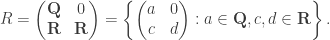
Finally, note that we’ve been talking about left modules throughout, but we can also define the concept of noetherian and artinian for right modules. [ Or just note that a right R-module is the same as a left Rop-module. ] You may be surprised to learn that a left noetherian ring is not necessarily right noetherian. In fact, here we have a ring which is left noetherian and left artinian, but neither right noetherian nor right artinian!
Proof
It’s not right artinian or right noetherian because it has right ideals of the form  where A is a subspace of R as a Q-vector space. It is easy to see that the collection of such subspaces has no maximal or minimal element.
On the other hand, R is a direct sum of left ideals

Clearly J is simple. And I has a simple submodule  and the resulting quotient is I/I’ is isomorphic to J. Since I’, I/I’ and J are simple, they’re noetherian and artinian. Thus R is left noetherian and left artinian. ♦


such that
is an abelian group together with a bilinear map
such that the following universal property holds:
there is a unique additive map
such that
for any
is called a pure tensor.


is a left R-module satisfying
is also R-linear in M, i.e.


as left R-modules.
, we have


as T-modules.
taking
is R-linear.
there is a unique S-module homomorphism
such that


![V^G := K[G] \otimes_{K[H]} V](https://s0.wp.com/latex.php?latex=V%5EG+%3A%3D+K%5BG%5D+%5Cotimes_%7BK%5BH%5D%7D+V&bg=ffffff&fg=333333&s=0&c=20201002)
![\text{Hom}_{K[H]}(V, W) = \text{Hom}_{K[G]}(V^G, W).](https://s0.wp.com/latex.php?latex=%5Ctext%7BHom%7D_%7BK%5BH%5D%7D%28V%2C+W%29+%3D+%5Ctext%7BHom%7D_%7BK%5BG%5D%7D%28V%5EG%2C+W%29.&bg=ffffff&fg=333333&s=0&c=20201002)

is an exact sequence of left R-modules, then for any right R-module M, we get an exact sequence of abelian groups:


 and
and  respectively. Then the tensor product
  In particular, it is of dimension mn over K. Now we can “multiply” elements of V and W to obtain an element of this new space, e.g.
 where 0≤i≤2, 0≤j≤3. However, defining the tensor product with respect to a chosen basis is rather unwieldy: we’d like a definition which only depends on V and W, and not the bases we picked.
 where V, W, X are vector spaces, such that
 such that the following
  , there is a unique linear map
  such that
  is called a pure tensor element.
 where U is the subspace generated by elements of the form:
 given by
  And v⊗w is the image of
  in T/U. ♦
 , where
  ;
; , where
  ;
; , where
  ;
; , where
  .
. taking
  Next we check that the map
 taking
  Similarly one defines a reverse map
  taking
  Since the pure tensors generate the whole space, it follows that f and g are mutually inverse.
 and
and  of vector spaces, we have:
 maps to
  on the RHS.
 and
and  are bases of V and W respectively, then
 forms a basis of V⊗W. This recovers our original intuitive definition of the tensor product!
 of V* where
 with the Kronecker delta symbol. The next result we would like to show is:
 taking (f, g) to the map
 taking (f, w) to the map
 taking
  is bilinear so it induces a map
  taking
  But the assignment (f, g) → h gives rise to a map
  which is bilinear so it induces
  Note that
  corresponds to the map
 and
and  of V* and W*. The map then takes
  to the linear map
  which takes
  to
to  But this corresponds to the dual basis of
  so we see that the above map φ takes a basis
  to a basis: dual of
 and
and  respectively. Then we form the column vector with mn entries
  This lets us see why V*⊗W* ≅ (V⊗W)*: in both cases we get a row vector with mn entries. Finally, to obtain V* ⊗W we take row vectors
 This gives an associative algebra over K by extending the bilinear map
 has basis
  , where we have shortened the notation
 etc.
etc. has basis
  , with 27 elements.
 gives
gives 


 This fails when the base ring is non-commutative because


 and covariant one by
  Breaking this convention will result in unnecessary confusion!
![R = \mathbf{Z}[a,b,c,d]/\left< ad-bc-1\right>.](https://s0.wp.com/latex.php?latex=R+%3D+%5Cmathbf%7BZ%7D%5Ba%2Cb%2Cc%2Cd%5D%2F%5Cleft%3C+ad-bc-1%5Cright%3E.&bg=ffffff&fg=333333&s=0&c=20201002)


 ♦
♦ is an
is an 
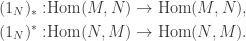
 is injective: if h : N → M’ is such that fh : N → M is zero, then since f is injective, h = 0.
 Thus
Thus 
 so h : N → M is a map such that gh : N → M” is the zero map. Then im(h) ⊆ ker(g) = im(f). Since f : M’ → M is injective, this gives
  and
and  ♦
♦ is an exact sequence. Then for any module N, we get an exact sequence:
 and a sequence of R-module homomorphisms:
 for all i.
 is exact if and only if f is injective.
 is exact if and only if g is surjective.
 is exact if and only if f is injective, g is surjective, and im(f) = ker(g). This is called a short exact sequence.
 for a submodule N of M. Short exact sequences are important because knowledge of N and M/N often tell us something about M itself. Here are some examples.
 , this allows us to break it into a collection of short exact sequences.
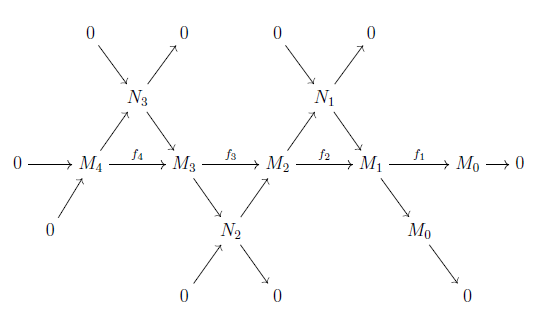

 We could repeat the same argument for the ranks of the terms, etc, but instead let’s have a common framework.
![\sum_{i=1}^k a_i [M_i],\quad a_i \in \mathbf{Z}, M_i \in \Sigma](https://s0.wp.com/latex.php?latex=%5Csum_%7Bi%3D1%7D%5Ek+a_i+%5BM_i%5D%2C%5Cquad+a_i+%5Cin+%5Cmathbf%7BZ%7D%2C+M_i+%5Cin+%5CSigma&bg=ffffff&fg=333333&s=0&c=20201002)
![\{[M_i] : M_i \in \Sigma\}.](https://s0.wp.com/latex.php?latex=%5C%7B%5BM_i%5D+%3A+M_i+%5Cin+%5CSigma%5C%7D.&bg=ffffff&fg=333333&s=0&c=20201002) Note that we specifically said ∑ is a set to avoid running into set-theoretic paradoxes. Take the quotient of this group by the subgroup generated by relations:
Note that we specifically said ∑ is a set to avoid running into set-theoretic paradoxes. Take the quotient of this group by the subgroup generated by relations:![[M] - [N] - [P]](https://s0.wp.com/latex.php?latex=%5BM%5D+-+%5BN%5D+-+%5BP%5D&bg=ffffff&fg=333333&s=0&c=20201002) if there is an exact sequence
if there is an exact sequence 

![[M_0] - [M_1] + \ldots + (-1)^{n-1}[M_{n-1}] + (-1)^n [M_n] = 0.](https://s0.wp.com/latex.php?latex=%5BM_0%5D+-+%5BM_1%5D+%2B+%5Cldots+%2B+%28-1%29%5E%7Bn-1%7D%5BM_%7Bn-1%7D%5D+%2B+%28-1%29%5En+%5BM_n%5D+%3D+0.&bg=ffffff&fg=333333&s=0&c=20201002)
![[M], M\in \Sigma\ \mapsto\ [N_0] + [N_1]+ \ldots + [N_k] \in \mathbf{Z}\Phi](https://s0.wp.com/latex.php?latex=%5BM%5D%2C+M%5Cin+%5CSigma%5C+%5Cmapsto%5C+%5BN_0%5D+%2B+%5BN_1%5D%2B+%5Cldots+%2B+%5BN_k%5D+%5Cin+%5Cmathbf%7BZ%7D%5CPhi&bg=ffffff&fg=333333&s=0&c=20201002)
 are the
  is unique, given that M is noetherian and artinian.
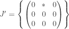
 be the ring of upper-triangular 2 × 2 real matrices. Consider the module M of column vectors R2, where R acts by matrix multiplication. Then M is not simple since it has a submodule spanned by (1, 0). But M is indecomposable since any submodule N ⊂ M which contains an (x, y) for y≠0 must be the whole M.
 is a local ring.

 : for any x∈M, we have
  so we can write
  But then
  ; clearly the second term lies in
  and the first term gives
  so it lies in
 : if
: if  lies in
  then we have
  which gives
  and so
 or
or  The former case says k is injective and hence an isomorphism, so we have the latter case kn=0. Thus fh = 1-k is invertible (since 1 + nilpotent = unit), so f is right-invertible. By symmetry, it is also left-invertible. ♦
 satisfy
  then N splits as
  Furthermore f is injective, thus M is a direct summand of N.
 for all i=1,…,k.
 after which we can apply induction on k.
 be the projection onto U1 and
  be the projection onto Vi. This gives
  and thus
  Since im(p) ⊆ U1 this restricts to a map
 , one of the αj is invertible, say α1. Let
  be the inverse of
  , so
, so where
where  (*)
(*) we write (*) as
 where
where 
 The second term is isomorphic to V1 and the first is just ker(p), which is
  as desired. ♦

 One sees that this is closed under addition (we need P to be prime so that the product of elements of S–P remains in S–P). So R is local with maximal ideal M.
 We saw in the

 of two-sided ideals must terminate so eventually
  Let J be this ideal; we get
  We need to show that J=0.
 for some n. Now each
  is a left-module annihilated by J so it is an (R/J)-module, i.e.
  A semisimple module is a direct sum of simple modules; if it is artinian, there are only finitely many terms in this direct sum, so it is noetherian too. Hence each


 is simple for each i=0,…,n-1. The length of the composition series is then n. The modules
  are called the composition factors of the series.
 with real entries. Let R act on M = R3 by left multiplication, so we get an R-module. We get a sequence of submodules:
 of submodules of M. Since M is noetherian this must terminate after finitely many terms. ♦
 such that the consecutive quotients are simple.
 and
and  are composition series of M with distinct composition factors;
 are the same submodule of M, then
  and
and  are composition series for this submodule with distinct composition factors, which contradicts the minimality of M.
 so we have
 (#)
(#) . Now pick a composition series (Pi) for
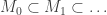
  We have:
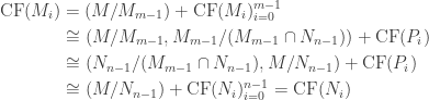
 are proper submodules, so any two composition series must have identical factors. Pictorially, we have:
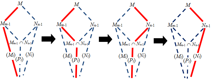
 which is isomorphic to I. Similarly, K has a submodule which is isomorphic to J. Hence, as composition factors, we can write:
 such that if N’ satisfies N ⊆ N’ ⊆ M, then N’=N or N’=M.
 , then the Z-module M/Z has no maximal submodule.
 of simple submodules
  For each index i, let
  be the submodule of M obtained by summing all
  Then each
  ♦
♦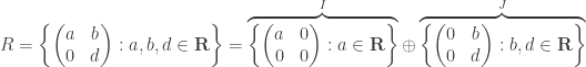
 which is isomorphic to I, and the quotient J/J’ is another simple module. Hence any simple module of R is isomorphic to I or J/J’.
 So this is J(R).
 We claim that there is a finite subset
  such that
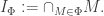
 has a minimal element, also written as
  If it is not zero, pick
  and since rad(R) = 0 there is an M∈∑ not containing x. But now
  is properly contained in
  contradicting its minimality. This proves our claim.
 is injective. Since R/M is simple, the RHS is semisimple (as R-modules) and hence R is also semisimple. ♦