
Introduction
Throughout this article, we let G be a subgroup of 

- Given A, how do we compute the order of G?
- How do we determine if an element
lies in G?
- Assuming
, how do we represent g as a product of elements of A and their inverses?
In general, the order of G is comparable to 
We will answer the first two questions in this article. The third is trickier, but there is a nice algorithm by Minkwitz which works for most practical instances.
Application
We can represent the group of transformations of the Rubik’s cube as a subgroup of 

[Image from official Rubik’s cube website.]
Our link above gives the exact order of the Rubik’s cube group (43252003274489856000), as computed by the open source algebra package GAP 4. How does it do that, without enumerating all the elements of the group? The answer will be given below.

Schreier-Sims Algorithm
To describe the Schreier-Sims algorithm, we use the following notations:
is some subset represented in the computer’s memory;
is a subgroup of
- G acts on the set
![[n] := \{1, 2, \ldots, n\}.](https://s0.wp.com/latex.php?latex=%5Bn%5D+%3A%3D+%5C%7B1%2C+2%2C+%5Cldots%2C+n%5C%7D.&bg=ffffff&fg=333333&s=0&c=20201002)
Let us pick some random element ![k\in [n]](https://s0.wp.com/latex.php?latex=k%5Cin+%5Bn%5D&bg=ffffff&fg=333333&s=0&c=20201002)


where 
Thus, if we could effectively obtain a set of generators for 
For that, we pick a set U of representatives for the left cosets 


Schreier Vector for Computing Orbits
Warning: our description of the Schreier vector differs slightly from the usual implementation, since we admit the inverse of a generator.
Let us label the elements of the generating set

- Initialize an array (v[1], v[2], …, v[n]) of integers to -1.
- Set v[k] := 0.
- For each i = 1, 2, …, n:
- If v[i] = -1 we ignore the next step.
- For each r = 1, 2, …, m, we set g = gr:
- set j := g(i); if v[j] = -1, then set v[j] = 2r-1;
- set j := g-1(i): if v[j] = -1, then set v[j] = 2r.
- Repeat the previous step until no more changes were made to v.
The idea is that v contains a “pointer” to an element of A (or its inverse) which brings it one step closer to k.
Example
Suppose we have elements

Labelling 


Thus the orbit of 1 is {1, 2, 3, 4, 5, 6, 7, 9}. To compute an element which maps 1 to, say, 9, the vector gives us 

Key Lemma
Next, we define the map 


Schreier’s Lemma.
The subgroup

Proof
First note that 


Next, observe that B is precisely the set of all 


Now suppose 

We will write

where 


So we have 

Example
Consider the subgroup 

If we pick k = 1, its orbit is 

Now the subgroup

Let 
Problem
The number of generators for the stabilizer groups seems to be ballooning: we started off with 2 examples, then expanded to 6 (but trimmed down to 4), then blew up to 20 after the second iteration.
Indeed, if we naively pick 


Thankfully, we have a way to pare down the number of generators.
Sims Filter
Sims Filter achieves the following.
Task.
Given a set
, there is an effective algorithm to replace
by some
satisfying
and

Let us explain the filter now. For any non-identity permutation 


Now we will construct a set B such that 


- Label
- Prepare a table indexed by (i, j) for all
. Initially this table is empty.
- For each
, if
we drop it.
- Otherwise, consider
. If the table entry at (i, j) is empty, we fill
in. Otherwise, if the entry is
, we replace
and repeat step 3.
- Note that this new group element takes i to i so if it is non-identity, we have
with
- Note that this new group element takes i to i so if it is non-identity, we have

After the whole process, the entries in the table give us the new set B. Clearly, we have
Example
As above, let us take A = {a, b} with

First step: since J(a) = (1, 5) we fill the element a in the table at (1, 5).
Second step: we also have J(b) = (1, 5), so now we have to replace b with

Now we have J(b’) = (2, 6) so this is allowed.
Summary and Applications
In summary, we denote 

- For i = 1, 2, …
- Pick a point
not picked earlier.
- Let
be the stabilizer group for
under the action of
From
, we use Schreier’s lemma to obtain a generating set for
- Use Sims filter to reduce this set to obtain
of at most
elements.
- If
- Pick a point

Thus ![k_1, k_2, \ldots, k_m \in [n] = \{1, 2, \ldots, n\}](https://s0.wp.com/latex.php?latex=k_1%2C+k_2%2C+%5Cldots%2C+k_m+%5Cin+%5Bn%5D+%3D+%5C%7B1%2C+2%2C+%5Cldots%2C+n%5C%7D&bg=ffffff&fg=333333&s=0&c=20201002)
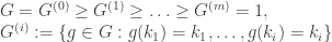
has an explicit set of generators of at most
1. Computing |G|.
It suffices to compute 


2. Determining if a given lies in G.
To check if 


Generalizing, we can determine if 

3. Checking if is a normal subgroup of 
Writing 


First we fix 


 modulo p tells us whether a is a square modulo p. We had written
  satisfies:
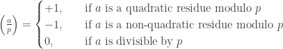


 and extend its definition to
  , we could compute
  and compare the two.

 is the Legendre symbol.


 and
and  it suffices to define, for positive odd m and n,
 and
and  The two claims are identical, so let’s just show the first, which is equivalent to:
 which is clearly even. ♦
 we repeatedly apply the above properties to obtain:
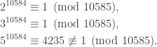
 and base
  , compute the Jacobi symbol
 . On the other hand,
  Thus even though n passes the Euler test for base 2, it fails the Solovay-Strassen test for the same base.
 but
but 
 We also saw that this method would utterly fail when we throw a Carmichael number at it.
 is prime and
  , then
 is a multiple of p and since p is prime either (m – 1) or (m + 1) is a multiple of p and the result follows.
 If it is not, then n is not prime. This is called the Euler test with base a.
 , then we must have

 Hence a pseudoprime can be picked up by the Euler test.

 instead of
  .
. is such that
  , then we say
 we have
  However, since
  is even, we can go one step further and check if
  In our case, we obtain
  and thus we see that n is composite.
 and the exponent
  is even, then we check whether
 be the highest power of 2 dividing
  and compute
 iterations.
 , output PASS.
 .
. , output FAIL.
 Thus we have
 Thus we skip step 3 as well.
 Thus step 3 says n fails the test.
 The next iteration then gives
  so n passes the Rabin-Miller test to base 2.
 for about 20 trials. If n passes all trials, we report that it is most likely prime. Otherwise, if it fails even a single trial, then it is composite. Heuristically, one imagines that the probability of n being composite and passing all trials to be about
  . In practice 75% is a gross underestimate since for most randomly chosen large n, the Rabin-Miller test will fail for >99% of the bases.
 , then it is prime.
 is generated by elements bounded by
  and thus it suffices to check for all bases in that bound. The conjecture remains open to this day – if you can prove it, you stand to win
 ![k\le [\sqrt n]](https://s0.wp.com/latex.php?latex=k%5Cle+%5B%5Csqrt+n%5D&bg=ffffff&fg=333333&s=0&c=20201002) .
.![[\sqrt n]](https://s0.wp.com/latex.php?latex=%5B%5Csqrt+n%5D&bg=ffffff&fg=333333&s=0&c=20201002) ? Because if n is divisible by some k, it is also divisible by n/k. Thus we may assume one of the factors to be at most
? Because if n is divisible by some k, it is also divisible by n/k. Thus we may assume one of the factors to be at most  . For example, given 103, we quickly find that it is prime since it is not divisible by 2, 3, …, 10.
 , then p is not prime. This is called the Fermat test with base a. As example 2 below shows, it has its flaws.

 , we check if
  Hence we have:
 , then we say
  (see
(see  then we say
  we have a
  -equivariant map
![\displaystyle \bigotimes_j \text{Alt}^{\mu_j} \mathbb{C}^n \to \bigotimes_i \text{Sym}^{\lambda_i} \mathbb{C}^n \subset\mathbb{C}[z_{i,j}]^{(\lambda_i)}, \quad e_T^\circ \mapsto D_T](https://s0.wp.com/latex.php?latex=%5Cdisplaystyle+%5Cbigotimes_j+%5Ctext%7BAlt%7D%5E%7B%5Cmu_j%7D+%5Cmathbb%7BC%7D%5En+%5Cto+%5Cbigotimes_i+%5Ctext%7BSym%7D%5E%7B%5Clambda_i%7D+%5Cmathbb%7BC%7D%5En+%5Csubset%5Cmathbb%7BC%7D%5Bz_%7Bi%2Cj%7D%5D%5E%7B%28%5Clambda_i%29%7D%2C+%5Cquad+e_T%5E%5Ccirc+%5Cmapsto+D_T&bg=ffffff&fg=333333&s=0&c=20201002)
 in both spaces. The kernel Q of this map is spanned by
  for various fillings T with shape
  and entries in [n].
 and
and  ; then
  and the map induces:
![\displaystyle \text{Alt}^3 \mathbb{C}^5 \otimes \text{Alt}^2 \mathbb{C}^5 \otimes \text{Alt}^2 \mathbb{C}^5\otimes \mathbb{C}^5 \longrightarrow \mathbb{C}[z_{1,j}]^{(4)} \otimes \mathbb{C}[z_{2,j}]^{(3)}\otimes \mathbb{C}[z_{3,j}]^{(1)}, \ 1\le j \le 5,](https://s0.wp.com/latex.php?latex=%5Cdisplaystyle+%5Ctext%7BAlt%7D%5E3+%5Cmathbb%7BC%7D%5E5+%5Cotimes+%5Ctext%7BAlt%7D%5E2+%5Cmathbb%7BC%7D%5E5+%5Cotimes+%5Ctext%7BAlt%7D%5E2+%5Cmathbb%7BC%7D%5E5%5Cotimes+%5Cmathbb%7BC%7D%5E5+%5Clongrightarrow%C2%A0%5Cmathbb%7BC%7D%5Bz_%7B1%2Cj%7D%5D%5E%7B%284%29%7D+%5Cotimes+%5Cmathbb%7BC%7D%5Bz_%7B2%2Cj%7D%5D%5E%7B%283%29%7D%5Cotimes+%5Cmathbb%7BC%7D%5Bz_%7B3%2Cj%7D%5D%5E%7B%281%29%7D%2C+%5C+1%5Cle+j+%5Cle+5%2C&bg=ffffff&fg=333333&s=0&c=20201002)

 , then the above map factors through
 .
. , then swapping columns
  and
and  of
of  gives us the same
  . ♦
. ♦ and
and  ; pick
  with length a. Now
  comprises of m copies of a so by the above lemma, we have a map:
![\displaystyle \text{Sym}^m \left(\text{Alt}^a \mathbb{C}^n\right) \longrightarrow \mathbb{C}[z_{1,j}]^{(m)} \otimes \ldots \otimes \mathbb{C}[z_{a,j}]^{(m)} \cong \mathbb{C}[z_{i,j}]^{(m,\ldots,m)}](https://s0.wp.com/latex.php?latex=%5Cdisplaystyle+%5Ctext%7BSym%7D%5Em+%5Cleft%28%5Ctext%7BAlt%7D%5Ea+%5Cmathbb%7BC%7D%5En%5Cright%29+%5Clongrightarrow+%5Cmathbb%7BC%7D%5Bz_%7B1%2Cj%7D%5D%5E%7B%28m%29%7D+%5Cotimes+%5Cldots+%5Cotimes+%5Cmathbb%7BC%7D%5Bz_%7Ba%2Cj%7D%5D%5E%7B%28m%29%7D%C2%A0%5Ccong+%5Cmathbb%7BC%7D%5Bz_%7Bi%2Cj%7D%5D%5E%7B%28m%2C%5Cldots%2Cm%29%7D&bg=ffffff&fg=333333&s=0&c=20201002)
 and
and  . Taking the direct sum over all m we have:
![\displaystyle \text{Sym}^* \left(\text{Alt}^a \mathbb{C}^n\right) := \bigoplus_{m\ge 0} \text{Sym}^m \left(\text{Alt}^a \mathbb{C}^n\right)\longrightarrow \bigoplus_{m\ge 0}\mathbb{C}[z_{i,j}]^{(m,\ldots,m)} \subset \mathbb{C}[z_{i,j}]](https://s0.wp.com/latex.php?latex=%5Cdisplaystyle+%5Ctext%7BSym%7D%5E%2A+%5Cleft%28%5Ctext%7BAlt%7D%5Ea+%5Cmathbb%7BC%7D%5En%5Cright%29+%3A%3D+%5Cbigoplus_%7Bm%5Cge+0%7D+%5Ctext%7BSym%7D%5Em+%5Cleft%28%5Ctext%7BAlt%7D%5Ea+%5Cmathbb%7BC%7D%5En%5Cright%29%5Clongrightarrow+%5Cbigoplus_%7Bm%5Cge+0%7D%5Cmathbb%7BC%7D%5Bz_%7Bi%2Cj%7D%5D%5E%7B%28m%2C%5Cldots%2Cm%29%7D+%5Csubset+%5Cmathbb%7BC%7D%5Bz_%7Bi%2Cj%7D%5D&bg=ffffff&fg=333333&s=0&c=20201002)
 for any vector space V has an algebra structure via
  The above map clearly preserves multiplication since multiplying
  and
and  both correspond to concatenation of T and T’. So it is also a homomorphism of
  -algebras.
 is given by
 Hence
Hence ![\text{Sym}^*\left(\text{Alt}^a \mathbb{C}^n\right) \cong \mathbb{C}[e_{i_1,\ldots,i_a}]](https://s0.wp.com/latex.php?latex=%5Ctext%7BSym%7D%5E%2A%5Cleft%28%5Ctext%7BAlt%7D%5Ea+%5Cmathbb%7BC%7D%5En%5Cright%29+%5Ccong+%5Cmathbb%7BC%7D%5Be_%7Bi_1%2C%5Cldots%2Ci_a%7D%5D&bg=ffffff&fg=333333&s=0&c=20201002) , the ring of polynomials in
, the ring of polynomials in  variables. What is the kernel
  of the induced map:
![\mathbb{C}[e_{i_1, \ldots, i_a}] \longrightarrow \mathbb{C}[z_{1,1}, \ldots, z_{a,n}]?](https://s0.wp.com/latex.php?latex=%5Cmathbb%7BC%7D%5Be_%7Bi_1%2C+%5Cldots%2C+i_a%7D%5D+%5Clongrightarrow+%5Cmathbb%7BC%7D%5Bz_%7B1%2C1%7D%2C+%5Cldots%2C+z_%7Ba%2Cn%7D%5D%3F&bg=ffffff&fg=333333&s=0&c=20201002)
 and
and  we have:
 with various sets of k indices in
  while preserving the order to give
  and
and  . Hence, P contains the ideal generated by all such quadratic relations.
 is a multiple of such a quadratic equation with a polynomial. This is clear by taking the two columns used in swapping; the remaining columns simply multiply the quadratic relation with a polynomial. Hence P is the ideal generated by these quadratic equations. ♦
![\mathbb{C}[e_{i_1, \ldots, i_a}]](https://s0.wp.com/latex.php?latex=%5Cmathbb%7BC%7D%5Be_%7Bi_1%2C+%5Cldots%2C+i_a%7D%5D&bg=ffffff&fg=333333&s=0&c=20201002) by
by ![\mathbb{C}[z_{i,j}]](https://s0.wp.com/latex.php?latex=%5Cmathbb%7BC%7D%5Bz_%7Bi%2Cj%7D%5D&bg=ffffff&fg=333333&s=0&c=20201002) , we have:
, we have: takes
takes  , which is a left action; here
  ,
,  . We also let
  act on the right via:
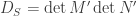
 -bimodule. A basic problem in invariant theory is to describe the ring
 ![\mathbb{C}[z_{i,j}]^{SL_a\mathbb{C}}](https://s0.wp.com/latex.php?latex=%5Cmathbb%7BC%7D%5Bz_%7Bi%2Cj%7D%5D%5E%7BSL_a%5Cmathbb%7BC%7D%7D&bg=ffffff&fg=333333&s=0&c=20201002) comprising of all f such that
comprising of all f such that  for all
  .
.![\displaystyle \mathbb{C}[D_{i_1, \ldots, i_a}] \cong \mathbb{C}[e_{i_1, \ldots, i_a}]/P \hookrightarrow \mathbb{C}[z_{i,j}]](https://s0.wp.com/latex.php?latex=%5Cdisplaystyle+%5Cmathbb%7BC%7D%5BD_%7Bi_1%2C+%5Cldots%2C+i_a%7D%5D+%5Ccong+%5Cmathbb%7BC%7D%5Be_%7Bi_1%2C+%5Cldots%2C+i_a%7D%5D%2FP+%5Chookrightarrow+%5Cmathbb%7BC%7D%5Bz_%7Bi%2Cj%7D%5D&bg=ffffff&fg=333333&s=0&c=20201002)
 runs over all
  -invariants in
 to:
to: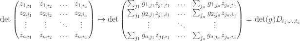
 . Hence we have
 ![\mathbb{C}[D_{i_1, \ldots, i_a}] \subseteq \mathbb{C}[z_{i,j}]^{SL_a\mathbb{C}}](https://s0.wp.com/latex.php?latex=%5Cmathbb%7BC%7D%5BD_%7Bi_1%2C+%5Cldots%2C+i_a%7D%5D%C2%A0%5Csubseteq+%5Cmathbb%7BC%7D%5Bz_%7Bi%2Cj%7D%5D%5E%7BSL_a%5Cmathbb%7BC%7D%7D&bg=ffffff&fg=333333&s=0&c=20201002) . To prove equality, we show that their dimensions in degree d agree. By the
. To prove equality, we show that their dimensions in degree d agree. By the ![\mathbb{C}[e_{i_1, \ldots, i_a}]/P](https://s0.wp.com/latex.php?latex=%5Cmathbb%7BC%7D%5Be_%7Bi_1%2C+%5Cldots%2C+i_a%7D%5D%2FP&bg=ffffff&fg=333333&s=0&c=20201002) has a basis indexed by SSYT of type
has a basis indexed by SSYT of type  and entries in [n]; if d is not a multiple of a, the component is 0.
![\mathbb{C}[z_{i,j}]^{SL_a\mathbb{C} }](https://s0.wp.com/latex.php?latex=%5Cmathbb%7BC%7D%5Bz_%7Bi%2Cj%7D%5D%5E%7BSL_a%5Cmathbb%7BC%7D+%7D&bg=ffffff&fg=333333&s=0&c=20201002) . As
. As ![\displaystyle \mathbb{C}[z_{i,j}] \cong \text{Sym}^*\left( (\mathbb{C}^a)^{\oplus n}\right)](https://s0.wp.com/latex.php?latex=%5Cdisplaystyle+%5Cmathbb%7BC%7D%5Bz_%7Bi%2Cj%7D%5D+%5Ccong+%5Ctext%7BSym%7D%5E%2A%5Cleft%28+%28%5Cmathbb%7BC%7D%5Ea%29%5E%7B%5Coplus+n%7D%5Cright%29&bg=ffffff&fg=333333&s=0&c=20201002)
 canonically. Taking the degree-d component, once again this component is 0 if d is not a multiple of a. If
  , it is the direct sum of
  over all
  . The
. The  of this submodule is
  where
where  is the sequence
  Hence
Hence
 and sum over all
  ; we see that the number of copies of
  is the number of SSYT with shape
  acts as a constant scalar on the whole of
  is homogeneous. Hence any
  is either the whole space or 0. From
  with a terms (which corresponds to
  ). Hence, the required dimension is the number of SSYT with shape
  and entries in [n]. ♦
 for
for  . For each sequence
  we define the following polynomials in
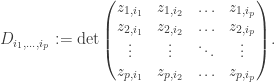

 is the sequence of entries from the i-th column of T. E.g.
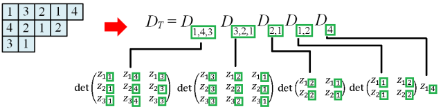
 with complex coefficients. Since we usually take entries of T from [n], we only need to consider the subring
 ![\mathbb{C}[z_{i,1}, \ldots, z_{i,n}]](https://s0.wp.com/latex.php?latex=%5Cmathbb%7BC%7D%5Bz_%7Bi%2C1%7D%2C+%5Cldots%2C+z_%7Bi%2Cn%7D%5D&bg=ffffff&fg=333333&s=0&c=20201002) .
. Recall
 be the element of
  obtained by replacing each entry k in T by
  , then taking the wedge of elements in each column, followed by the tensor product across columns:
 is precisely
  as defined in the

 of degree 5,
  of degree 4 and
  of degree 3. We let
  act on
 as a row vector, then
  . From another point of view, if we take
  as a basis, then the action is represented by matrix g since it takes the standard basis to the column vectors of g.
 takes
takes  by taking the column vectors of g; so
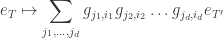
 with
with  correspondingly.
 gets mapped to:
 . ♦
. ♦ The resulting quotient is thus identical to the Schur module F(V), and the above map factors through
 if T has two identical entries in the same column.
 if T’ is obtained from T by swapping two entries in the same column.
 , where S takes the set of all fillings obtained from T by swapping a fixed set of k entries in column j’ with arbitrary sets of k entries in column j (for fixed j < j’) while preserving the order.
 Now apply the above linear map. ♦
 . Writing out the third relation in corollary 1 gives:
![\left[\det\begin{pmatrix} a & c \\ b & d\end{pmatrix}\right] x = \left[\det\begin{pmatrix} x & c \\ y & d\end{pmatrix}\right] a + \left[ \det\begin{pmatrix} a & x \\ b & y\end{pmatrix}\right] c.](https://s0.wp.com/latex.php?latex=%5Cleft%5B%5Cdet%5Cbegin%7Bpmatrix%7D+a+%26+c+%5C%5C+b+%26+d%5Cend%7Bpmatrix%7D%5Cright%5D+x+%3D+%5Cleft%5B%5Cdet%5Cbegin%7Bpmatrix%7D+x+%26+c+%5C%5C+y+%26+d%5Cend%7Bpmatrix%7D%5Cright%5D+a+%2B+%5Cleft%5B+%5Cdet%5Cbegin%7Bpmatrix%7D+a+%26+x+%5C%5C+b+%26+y%5Cend%7Bpmatrix%7D%5Cright%5D+c.&bg=ffffff&fg=333333&s=0&c=20201002)
 and
and  , the corresponding third relation is obtained by multiplying the above by a polynomial on both sides.
 SYT by writing
  in the left column and
  in the right. Now
  is the product:
 , where matrices M’, N’ are obtained from M, N respectively by swapping a fixed set of k columns in N with arbitrary sets of k columns in M while preserving the column order. E.g. for n=3 and k=2, picking the first two columns of N gives:
 , one takes its Young diagram comprising of boxes. A filling is given by a function
 ![T:\lambda \to [m]](https://s0.wp.com/latex.php?latex=T%3A%5Clambda+%5Cto+%5Bm%5D&bg=ffffff&fg=333333&s=0&c=20201002) for some positive integer m. When m=d, we will require the filling to be bijective, i.e. T contains {1,…,d} and each element occurs exactly once.
for some positive integer m. When m=d, we will require the filling to be bijective, i.e. T contains {1,…,d} and each element occurs exactly once. and
and  is obtained by replacing each i in the filling with w(i). For a filling T, the corresponding row (resp. column) tabloid is denoted by {T} (resp. [T]).
 -irrep
  as a quotient of
 ![\mathbb{C}[S_d]b_{T_0}](https://s0.wp.com/latex.php?latex=%5Cmathbb%7BC%7D%5BS_d%5Db_%7BT_0%7D&bg=ffffff&fg=333333&s=0&c=20201002) from the surjection:
from the surjection:![\mathbb{C}[S_d] b_{T_0} \to \mathbb{C}[S_d] b_{T_0} a_{T_0}, \quad v \mapsto v a_{T_0}.](https://s0.wp.com/latex.php?latex=%5Cmathbb%7BC%7D%5BS_d%5D+b_%7BT_0%7D+%5Cto+%5Cmathbb%7BC%7D%5BS_d%5D+b_%7BT_0%7D+a_%7BT_0%7D%2C+%5Cquad+v+%5Cmapsto+v+a_%7BT_0%7D.&bg=ffffff&fg=333333&s=0&c=20201002)
 is any fixed bijective filling
 ![\lambda \to [d]](https://s0.wp.com/latex.php?latex=%5Clambda+%5Cto+%5Bd%5D&bg=ffffff&fg=333333&s=0&c=20201002) .
.![[T] = \sum_{T'} [T']](https://s0.wp.com/latex.php?latex=%5BT%5D+%3D+%5Csum_%7BT%27%7D+%5BT%27%5D&bg=ffffff&fg=333333&s=0&c=20201002) where T’ runs through all column tabloids obtained from T as follows:
where T’ runs through all column tabloids obtained from T as follows:
![V(\lambda) = V^{\otimes d} \otimes_{\mathbb{C}[S_d]} V_\lambda](https://s0.wp.com/latex.php?latex=V%28%5Clambda%29+%3D+V%5E%7B%5Cotimes+d%7D+%5Cotimes_%7B%5Cmathbb%7BC%7D%5BS_d%5D%7D+V_%5Clambda&bg=ffffff&fg=333333&s=0&c=20201002) , where
, where  be the set of all functions
  , i.e. the set of all fillings of λ with elements of V. We define the map:
![\Psi : V^{\times\lambda} \to V^{\otimes d}\otimes_{\mathbb{C}[S_d]} V_\lambda, \quad (v_s)_{s\in\lambda} \mapsto \overbrace{\left[v_{T^{-1}(1)} \otimes \ldots \otimes v_{T^{-1}(d)}\right]}^{\in V^{\otimes d}} \otimes [T]](https://s0.wp.com/latex.php?latex=%5CPsi+%3A+V%5E%7B%5Ctimes%5Clambda%7D+%5Cto+V%5E%7B%5Cotimes+d%7D%5Cotimes_%7B%5Cmathbb%7BC%7D%5BS_d%5D%7D+V_%5Clambda%2C+%5Cquad+%28v_s%29_%7Bs%5Cin%5Clambda%7D+%5Cmapsto+%5Coverbrace%7B%5Cleft%5Bv_%7BT%5E%7B-1%7D%281%29%7D+%5Cotimes+%5Cldots+%5Cotimes+v_%7BT%5E%7B-1%7D%28d%29%7D%5Cright%5D%7D%5E%7B%5Cin+V%5E%7B%5Cotimes+d%7D%7D+%5Cotimes+%5BT%5D&bg=ffffff&fg=333333&s=0&c=20201002)
![T:\lambda \to [d].](https://s0.wp.com/latex.php?latex=T%3A%5Clambda+%5Cto+%5Bd%5D.&bg=ffffff&fg=333333&s=0&c=20201002) This is independent of the T we pick; indeed if we replace T by
This is independent of the T we pick; indeed if we replace T by  , the resulting RHS would be:
![\begin{aligned}\left[v_{T^{-1}w^{-1}(1)} \otimes \ldots \otimes v_{T^{-1}w^{-1}(d)}\right] \otimes [w(T)] &= \left[v_{T^{-1}w^{-1}(1)}\otimes \ldots \otimes v_{T^{-1} w^{-1}(d)}\right]w \otimes [T]\\ &= \left[v_{T^{-1}(1)} \otimes \ldots \otimes v_{T^{-1}(d)}\right] \otimes [T]\end{aligned}](https://s0.wp.com/latex.php?latex=%5Cbegin%7Baligned%7D%5Cleft%5Bv_%7BT%5E%7B-1%7Dw%5E%7B-1%7D%281%29%7D+%5Cotimes+%5Cldots+%5Cotimes+v_%7BT%5E%7B-1%7Dw%5E%7B-1%7D%28d%29%7D%5Cright%5D+%5Cotimes+%5Bw%28T%29%5D+%26%3D+%5Cleft%5Bv_%7BT%5E%7B-1%7Dw%5E%7B-1%7D%281%29%7D%5Cotimes+%5Cldots+%5Cotimes+v_%7BT%5E%7B-1%7D+w%5E%7B-1%7D%28d%29%7D%5Cright%5Dw+%5Cotimes+%5BT%5D%5C%5C+%26%3D+%5Cleft%5Bv_%7BT%5E%7B-1%7D%281%29%7D+%5Cotimes+%5Cldots+%5Cotimes+v_%7BT%5E%7B-1%7D%28d%29%7D%5Cright%5D+%5Cotimes+%5BT%5D%5Cend%7Baligned%7D&bg=ffffff&fg=333333&s=0&c=20201002)
![\mathbb{C}[S_d]](https://s0.wp.com/latex.php?latex=%5Cmathbb%7BC%7D%5BS_d%5D&bg=ffffff&fg=333333&s=0&c=20201002) and the second equality follows from our definition
and the second equality follows from our definition  . Hence
  is well-defined. It satisfies the following three properties.
 and consider
  , then the resulting map is C-linear. E.g. if
  , then:
 are identical except
  and
and  , where
  are in the same column. Then
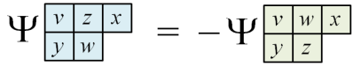
![w([T]) = -[T]](https://s0.wp.com/latex.php?latex=w%28%5BT%5D%29+%3D+-%5BT%5D&bg=ffffff&fg=333333&s=0&c=20201002) by alternating property of the column tabloid and
by alternating property of the column tabloid and  . Thus:
![\begin{aligned}\left[v'_{T^{-1}(1)} \otimes \ldots \otimes v'_{T^{-1}(d)}\right] \otimes [T] &= \left[ v_{T^{-1}w^{-1}(1)} \otimes \ldots \otimes v_{T^{-1}w^{-1}(d)}\right] \otimes -w([T])\\ &= -\left[v_{T^{-1}(1)} \otimes\ldots \otimes v_{T^{-1}(d)}\right]\otimes [T]. \end{aligned}](https://s0.wp.com/latex.php?latex=%5Cbegin%7Baligned%7D%5Cleft%5Bv%27_%7BT%5E%7B-1%7D%281%29%7D+%5Cotimes+%5Cldots+%5Cotimes+v%27_%7BT%5E%7B-1%7D%28d%29%7D%5Cright%5D+%5Cotimes+%5BT%5D+%26%3D+%5Cleft%5B+v_%7BT%5E%7B-1%7Dw%5E%7B-1%7D%281%29%7D+%5Cotimes+%5Cldots+%5Cotimes+v_%7BT%5E%7B-1%7Dw%5E%7B-1%7D%28d%29%7D%5Cright%5D+%5Cotimes+-w%28%5BT%5D%29%5C%5C+%26%3D+-%5Cleft%5Bv_%7BT%5E%7B-1%7D%281%29%7D+%5Cotimes%5Cldots+%5Cotimes+v_%7BT%5E%7B-1%7D%28d%29%7D%5Cright%5D%5Cotimes+%5BT%5D.+%5Cend%7Baligned%7D&bg=ffffff&fg=333333&s=0&c=20201002) ♦
♦ Fix two columns
  in the Young diagram for λ, and a set B of k boxes in column j’. As A runs through all sets of k boxes in column j, let
  be obtained by swapping entries in A with entries in B while
 we have:
![\begin{aligned}\Psi((v_s^A)) &= \left[v_{T^{-1}(1)}^A \otimes \ldots \otimes v_{T^{-1}(d)}^A\right] \otimes [T ]\\ &= \left[v_{T^{-1}w^{-1}(1)} \otimes \ldots \otimes v_{T^{-1}w^{-1}(d)}\right] \otimes [T] \\ &= \left[v_{T^{-1}(1)} \otimes \ldots \otimes v_{T^{-1}(d)}\right] \otimes w([T])\end{aligned}](https://s0.wp.com/latex.php?latex=%5Cbegin%7Baligned%7D%5CPsi%28%28v_s%5EA%29%29+%26%3D+%5Cleft%5Bv_%7BT%5E%7B-1%7D%281%29%7D%5EA+%5Cotimes+%5Cldots+%5Cotimes+v_%7BT%5E%7B-1%7D%28d%29%7D%5EA%5Cright%5D+%5Cotimes+%5BT+%5D%5C%5C+%26%3D+%5Cleft%5Bv_%7BT%5E%7B-1%7Dw%5E%7B-1%7D%281%29%7D+%5Cotimes+%5Cldots+%5Cotimes+v_%7BT%5E%7B-1%7Dw%5E%7B-1%7D%28d%29%7D%5Cright%5D+%5Cotimes+%5BT%5D+%5C%5C+%26%3D+%5Cleft%5Bv_%7BT%5E%7B-1%7D%281%29%7D+%5Cotimes+%5Cldots+%5Cotimes+v_%7BT%5E%7B-1%7D%28d%29%7D%5Cright%5D+%5Cotimes+w%28%5BT%5D%29%5Cend%7Baligned%7D&bg=ffffff&fg=333333&s=0&c=20201002)
 ). But the sum of all such
 ![w([T])](https://s0.wp.com/latex.php?latex=w%28%5BT%5D%29&bg=ffffff&fg=333333&s=0&c=20201002) vanishes in
vanishes in  Hence
Hence  ♦
♦ is said to be λ-alternating if properties C1, C2 and C3 hold.
 where
where is a λ-alternating map,
 to a complex vector space W, there is a unique linear map
  such that

 with a set A of coordinates in
  , and letting A vary over all |A| = |B|. E.g. the relation corresponding to our above example for C3 is:
![\begin{aligned} &\left[ (u\wedge x\wedge z) \otimes (v\wedge y) \otimes w\right] -\left[ (u\wedge y\wedge z) \otimes (u\wedge x) \otimes w\right] \\ - &\left[ (v\wedge x\wedge y)\otimes (u\wedge z)\otimes w\right] - \left[ (u\wedge x\wedge w) \otimes (v\wedge z) \otimes w\right]\end{aligned}](https://s0.wp.com/latex.php?latex=%5Cbegin%7Baligned%7D+%26%5Cleft%5B+%28u%5Cwedge+x%5Cwedge+z%29+%5Cotimes+%28v%5Cwedge+y%29+%5Cotimes+w%5Cright%5D+-%5Cleft%5B+%28u%5Cwedge+y%5Cwedge+z%29+%5Cotimes+%28u%5Cwedge+x%29+%5Cotimes+w%5Cright%5D+%5C%5C+-+%26%5Cleft%5B+%28v%5Cwedge+x%5Cwedge+y%29%5Cotimes+%28u%5Cwedge+z%29%5Cotimes+w%5Cright%5D+-+%5Cleft%5B+%28u%5Cwedge+x%5Cwedge+w%29+%5Cotimes+%28v%5Cwedge+z%29+%5Cotimes+w%5Cright%5D%5Cend%7Baligned%7D&bg=ffffff&fg=333333&s=0&c=20201002)

![\Psi: V^{\times\lambda} \to V^{\otimes d} \otimes_{\mathbb{C}[S_d]} V_\lambda](https://s0.wp.com/latex.php?latex=%5CPsi%3A+V%5E%7B%5Ctimes%5Clambda%7D+%5Cto+V%5E%7B%5Cotimes+d%7D+%5Cotimes_%7B%5Cmathbb%7BC%7D%5BS_d%5D%7D+V_%5Clambda&bg=ffffff&fg=333333&s=0&c=20201002) thus induces a linear:
thus induces a linear:![\alpha: F(V) \longrightarrow V^{\otimes d} \otimes_{\mathbb{C}[S_d]} V_\lambda.](https://s0.wp.com/latex.php?latex=%5Calpha%3A+F%28V%29+%5Clongrightarrow+V%5E%7B%5Cotimes+d%7D+%5Cotimes_%7B%5Cmathbb%7BC%7D%5BS_d%5D%7D+V_%5Clambda.&bg=ffffff&fg=333333&s=0&c=20201002)
 is an isomorphism.
![V^{\otimes d}\otimes_{\mathbb{C}[S_d]}V_\lambda \cong V(\lambda)](https://s0.wp.com/latex.php?latex=V%5E%7B%5Cotimes+d%7D%5Cotimes_%7B%5Cmathbb%7BC%7D%5BS_d%5D%7DV_%5Clambda+%5Ccong+V%28%5Clambda%29&bg=ffffff&fg=333333&s=0&c=20201002) , and we
, and we  be the standard basis of
  If T is any filling with shape λ and entries in [n], we let
  ; then running through the map

 in which
  , we have
  .
.
 for S > T.
 by definition.
 , assume j is the rightmost column for which this happens, and in that column, i is as large as possible. Swapping entries
  of T gives us T’ > T and
 , where j is the largest for which this happens, and
  , for
, for  . Swapping the topmost i entries of column j+1, with various i entries of column j, all the resulting fillings are strictly greater than T. Hence
  , where each S > T.
 ≤ number of SSYT with shape λ and entries in [n], and the proof for the main theorem is complete. From our proof, we have also obtained:
 forms a basis for F(V), where T runs through the set of all SSYT with shape λ and entries in [n].
 throughout this article. In the previous article, we saw that the

 and is called the Schur functor when M is fixed.
 induces a linear
  .
.![M = \mathbb{C}[S_d]](https://s0.wp.com/latex.php?latex=M+%3D+%5Cmathbb%7BC%7D%5BS_d%5D&bg=ffffff&fg=333333&s=0&c=20201002) , the functor
, the functor  is the identity functor. By Schur-Weyl duality, when M is irreducible as an
  is either 0 or irreducible. We will see the Schur functor cropping up in two other instances.
 ,
,
 must induce an isomorphism between those two components. We proceed to construct such a map.
 and pick the following filling:
 and
and  as subspaces of
  Thus:
Thus:
 according to the above filling, i.e.
  goes into components 1, 4, 2 of
  while
while  by mapping components 1, 3 to
  , components 4 and 2 to the other two copies of V. In diagram, we have:
 is a linear map of vector spaces, then this induces a linear map
 on the left and
![V(M) := V^{\otimes d} \otimes_{\mathbb{C}[G]} M,](https://s0.wp.com/latex.php?latex=V%28M%29+%3A%3D+V%5E%7B%5Cotimes+d%7D+%5Cotimes_%7B%5Cmathbb%7BC%7D%5BG%5D%7D+M%2C&bg=ffffff&fg=333333&s=0&c=20201002)
 corresponds to the Schur-Weyl duality, i.e.
  Once again, by additivity, we only need to consider the case
 ![M = \mathbb{C}[X_\lambda]](https://s0.wp.com/latex.php?latex=M+%3D+%5Cmathbb%7BC%7D%5BX_%5Clambda%5D&bg=ffffff&fg=333333&s=0&c=20201002) . This gives
. This gives ![M \cong \mathbb{C}[G]a_T](https://s0.wp.com/latex.php?latex=M+%5Ccong+%5Cmathbb%7BC%7D%5BG%5Da_T&bg=ffffff&fg=333333&s=0&c=20201002) where T is any filling of shape λ and thus:
where T is any filling of shape λ and thus:![V(M) = V^{\otimes d} \otimes_{\mathbb{C}[G]} \mathbb{C}[G]a_T \cong V^{\otimes d}a_T.](https://s0.wp.com/latex.php?latex=V%28M%29+%3D+V%5E%7B%5Cotimes+d%7D+%5Cotimes_%7B%5Cmathbb%7BC%7D%5BG%5D%7D+%5Cmathbb%7BC%7D%5BG%5Da_T+%5Ccong+V%5E%7B%5Cotimes+d%7Da_T.&bg=ffffff&fg=333333&s=0&c=20201002)
 and so
  is yet another expression of the Schur functor.
![\mathbb{C}[S_d]c_T](https://s0.wp.com/latex.php?latex=%5Cmathbb%7BC%7D%5BS_d%5Dc_T&bg=ffffff&fg=333333&s=0&c=20201002) where
where  is the Young symmetrizer for a fixed filling of shape λ. Hence, the irrep
 ![V^{\otimes d} \otimes_{\mathbb{C}[G]} V_\lambda \cong V^{\otimes d}\otimes_{\mathbb{C}[G]} \mathbb{C}[G]c_T \cong V^{\otimes d}c_T.](https://s0.wp.com/latex.php?latex=V%5E%7B%5Cotimes+d%7D+%5Cotimes_%7B%5Cmathbb%7BC%7D%5BG%5D%7D+V_%5Clambda+%5Ccong+V%5E%7B%5Cotimes+d%7D%5Cotimes_%7B%5Cmathbb%7BC%7D%5BG%5D%7D+%5Cmathbb%7BC%7D%5BG%5Dc_T+%5Ccong+V%5E%7B%5Cotimes+d%7Dc_T.&bg=ffffff&fg=333333&s=0&c=20201002)
 , let us take the Young symmetrizer:
 , then
  is spanned by elements of the form:

 with
with  . By the second relation, we may further restrict to the case
  since if
  we have
  and if
  we replace
 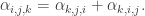 We claim that the resulting spanning set
  forms a basis. Indeed the number of such triplets (i, j, k) is:
 has one copy of
  , one copy of
  and two copies of
 is the cardinality of the set and we are done. ♦
![\{(i,j,k) \in [n]^d : i\le j, i<k\}](https://s0.wp.com/latex.php?latex=%5C%7B%28i%2Cj%2Ck%29+%5Cin+%5Bn%5D%5Ed+%3A+i%5Cle+j%2C+i%3Ck%5C%7D&bg=ffffff&fg=333333&s=0&c=20201002) corresponds to the set of all SSYT with shape (2, 1) and entries in [n] (by writing i, j in the first row and k below i). This is an example of our
corresponds to the set of all SSYT with shape (2, 1) and entries in [n] (by writing i, j in the first row and k below i). This is an example of our  in the next article. This corresponds to an
 ![\mathbb{C}[S_d]b_T](https://s0.wp.com/latex.php?latex=%5Cmathbb%7BC%7D%5BS_d%5Db_T&bg=ffffff&fg=333333&s=0&c=20201002) .
. for convenience.
 of degree d and representations of
  and polynomial representations of
  .
. Recall from earlier, that
 as endomorphisms of
  of all elements fixed by every
 , consider the binomial expansion in
 matrix with (i, j)-entry
  (where
  ) has rank d+1.
 , not all zero, such that
  for all large k, which is absurd since this is a polynomial in k.
 lies in the subspace spanned by all
  . By induction hypothesis, the set of all
  spans the whole space. Hence, the set of all
  is an
is an  .
. we have
  Hence from the given condition
 for all
  Since
Since  is dense, f is also a linear combination of
  . ♦
. ♦ Recall: if
  is any subset,
 is a subalgebra and we have
 is semisimple;
 ; (double centralizer theorem)
 , where
  are respectively complete lists of irreducible A-modules and B-modules.
 . Each simple A-module is of the form
  for some
  As an A-module, we can decompose:
  Here
Here  since as A-modules we have:
 if
if  and 0 otherwise. This gives:
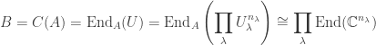
 has dimension
  . From the action of B on U, we can write
  where A acts on the
  and B acts on the
  ; thus repeating the above with A replaced by B gives:
 we thus have
  This proves all three properties. ♦
 as complex vector spaces,
 acts on the
 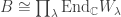 acts on the
 This functor is additive, i.e.
  , since the Hom functor is bi-additive.
 . Now A is semisimple since it is a quotient of
 .
.![\mathbb{C}[X_\lambda]](https://s0.wp.com/latex.php?latex=%5Cmathbb%7BC%7D%5BX_%5Clambda%5D&bg=ffffff&fg=333333&s=0&c=20201002) corresponds to
corresponds to  via the functor in the above note, then
![W' = \text{Hom}_{S_d}(\mathbb{C}[X_\lambda], V^{\otimes d}).](https://s0.wp.com/latex.php?latex=W%27+%3D%C2%A0%5Ctext%7BHom%7D_%7BS_d%7D%28%5Cmathbb%7BC%7D%5BX_%5Clambda%5D%2C+V%5E%7B%5Cotimes+d%7D%29.&bg=ffffff&fg=333333&s=0&c=20201002) Recall that
Recall that  is a transitive
  , any map
 ![f:\mathbb{C}[X_\lambda] \to V^{\otimes d}](https://s0.wp.com/latex.php?latex=f%3A%5Cmathbb%7BC%7D%5BX_%5Clambda%5D+%5Cto+V%5E%7B%5Cotimes+d%7D&bg=ffffff&fg=333333&s=0&c=20201002) which is
which is  , as long as this element is invariant under the stabilizer group:
 of
of  in
in  remain invariant when acted upon by
  . So we have an element of
  ♦
♦


 so
so 
 is trivial on the first component and alternating on the second.
 is of the form
  such that
  is the Schur polynomial
  .
. for an integer k. Then:
 . What is this
  ). Hence from
  we must have
  Thus:
Thus:

 ,
,  so the representation
  is polynomial if and only if
  Its degree is
 for some partition
  and integer k. From:
 in lexicographical order. For large N, denoting
  for the reverse of a sequence
 and
and  Pictorially we have:
 , as vector spaces we have:
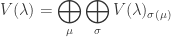
 and
and  ;
; runs through all permutations of
  we get 3 terms: (5, 3, 3), (3, 5, 3) and (3, 3, 5);
 is the space of all
  for which S acts with character
  , i.e.
 . This is called the weight space decomposition of
  is exactly the number of SSYT with shape
  over all SSYT T of shape
  lies in the space
 By the above proposition, each irreducible representation is given by
  where m, k are integers and
  To compute V(m), we need to find a polynomial representation of G such that
 from:
from:
 ; if {e, f} is a basis of V, then a corresponding basis of
  . If
. If  , then the diagonal matrix D(a, b) takes
  so its character is
  as desired.
 is 1-dimensional and spanned by
 . We have:

 and
and  , both
  and
and  are irreps of G. The weight space decomposition of the two spaces are:
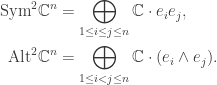
 and compute
  and
and  To find
  we need to compute
  for all
  and
and  We will work in the plane
  since partitions lie in the region
  , we only consider the coloured region:
 . Assuming
  , the condition
  then reduces to a single inequality
  Hence,
 Calculating the Kostka coefficients gives us:

 and
and  . These correspond to the following SSYT of shape (5,3):
