Polynomials and Representations XXXIV | Mathematics and Such

Polynomials and Representations XXXIV

Posted on June 25, 2016 by limsup

Twisting

From the previous article, any irreducible polynomial representation of $G= GL_n\mathbb{C}$ is of the form $V(\lambda)$ for some $\lambda \vdash d, l(\lambda) \le n$ such that $\psi_{V(\lambda)}$ is the Schur polynomial $s_\lambda(x_1, \ldots, x_n)$ .

Now given any analytic representation V of G, we can twist it by taking $V\otimes \det^k$ for an integer k. Then:

$\displaystyle\psi_{V \otimes \det^k}= \psi_V \cdot \psi_{\det}^k = (x_1 \ldots x_n)^k \psi_V.$

Twisting the irrep $V(\lambda)$ with $k\ge 0$ gives us another irrep, necessarily of the form $V(\mu)$ . What is this $\mu$ ? Note that from $\psi_{V(\lambda)}$ we can recover the partition $\lambda$ by taking the minimal partition (with respect to $\trianglelefteq$ ). Hence from $\psi_{V(\mu)} = (x_1\ldots x_n)^k\psi_{V(\lambda)}$ we must have $\mu = \lambda + (k, \ldots, k).$ Thus:

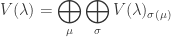
Proposition. Any irreducible analytic representation of G can be uniquely written as:

$\{\psi_{V(\lambda)} \otimes \det^k : l(\lambda) \le n-1, k\in\mathbb{Z}\}$

where $V(\lambda)$ is the polynomial representation satisfying:

$\psi_{V(\lambda)} = s_\lambda(x_1, \ldots, x_n).$

Since $l(\lambda) \le n-1$ , $s_\lambda(x_1, \ldots, x_n)$ is not divisible by $x_n$ so the representation $V(\lambda) \otimes \det^k$ is polynomial if and only if $k\ge 0.$ Its degree is $|\lambda| + kn.$

blue-lin

Dual of Irrep

The dual of the irrep $V(\lambda)$ is also a rational irrep, so it is of the form $V(\mu) \otimes \det^k$ for some partition $\mu$ with $l(\mu) \le n-1$ and integer k. From:

$\psi_{V(\lambda)^\vee}(x_1, \ldots, x_n) = \psi_{V(\lambda)}(x_1^{-1}, \ldots, x_n^{-1})$

we take the term with the smallest exponent for $x^\mu$ in lexicographical order. For large N, denoting $\text{rev}(\alpha)$ for the reverse of a sequence $\alpha$ , we have:

$\lambda, \mu \vdash d, \lambda \trianglerighteq \mu \implies \text{rev}((N,\ldots, N) - \lambda) \trianglerighteq \text{rev}((N,\ldots, N) - \mu).$

Hence $\mu = (\lambda_1, \lambda_1 - \lambda_{n-1}, \lambda_1 - \lambda_{n-2}, \ldots, \lambda_1 - \lambda_2)$ and $k = -\lambda_1.$ Pictorially we have:

partition_of_dual_representation

Weight Space Decomposition

By definition $\psi_{V(\lambda)}$ is the character of $V(\lambda)$ when acted upon by the torus group S. Since this polynomial is $s_\lambda = \sum_{\mu} K_{\lambda\mu} m_\mu$ , as vector spaces we have:

$\displaystyle V(\lambda) = \bigoplus_{\mu} \bigoplus_{\sigma} V(\lambda)_{\sigma(\mu)}$

where:

$\mu$ runs through all partitions with $|\mu| = |\lambda|$ and $l(\mu) \le n$ ;
$\sigma(\mu)$ runs through all permutations of $\mu$ without repetition, e.g. if $\mu = (5, 3, 3)$ we get 3 terms: (5, 3, 3), (3, 5, 3) and (3, 3, 5);
$V(\lambda)_{\nu}$ is the space of all $v\in V(\lambda)$ for which S acts with character $x^\nu$ , i.e.

$V(\lambda)_{\nu} = \{v \in V(\lambda) : D(x_1, \ldots, x_n) \in S \text{ takes } v\mapsto x^\nu v\}$

and the dimension of $V(\lambda)_{\nu}$ is $K_{\lambda\nu}$ . This is called the weight space decomposition of $V(\lambda).$ We will go through some explicit examples later.

Foreshadowing: SSYTs as a Basis

As noted above, the dimension of $V(\lambda)_{\sigma(\mu)}$ is exactly the number of SSYT with shape $\lambda$ and type $\sigma(\mu)$ . Thus in a somewhat ambiguous way, we can take, as a basis of $V(\lambda)$ , elements of the form $\{v_T\}$ over all SSYT T of shape $\lambda$ and entries from [n]={1,2,…,n}; each $v_T$ lies in the space $V(\lambda)_{\text{shape}(T)}.$

However, such a description does not distinguish between distinct SSYT of the same type. For that, one needs a construction like the determinant modules (to be described later).

blue-lin

Example: n=2

Consider $G = GL_2\mathbb C.$ By the above proposition, each irreducible representation is given by $V(m) \otimes \det^k$ where m, k are integers and $m\ge 0.$ To compute V(m), we need to find a polynomial representation of G such that

$\psi_{V(m)} = s_m(x, y)= x^m + x^{m-1}y + \ldots + y^m$

corresponding to the SSYT with shape (m) and entries comprising of only 1’s and 2’s. E.g. $s_4(x,y) = x^4 + x^3 y + x^2 y^2 + xy^3 + y^4$ from:

gl2_example_ssyt

Such a V(m) is easy to construct: take $\text{Sym}^m V$ ; if {e, f} is a basis of V, then a corresponding basis of $\text{Sym}^m V$ is given by $\{e^i f^{4-i}\}_{i=0,\ldots,4}$ . If $v_i := e^{2+i} f^{2-i}$ , then the diagonal matrix D(a, b) takes $v_i \mapsto a^{2+i} b^{2-i} v_i$ so its character is $a^4 + a^3 b + a^2 b^2 + ab^3 + b^4$ as desired.

The weight space decomposition thus gives:

$V(m) = V(m)_{4,0} \oplus V(m)_{3,1} \oplus V(m)_{2,2} \oplus V(m)_{1,3} \oplus V(m)_{0,4}$

where each $V(m)_{i,j}$ is 1-dimensional and spanned by $e^i f^{4-i}.$

Example: d=2

Consider $G = GL_n\mathbb{C}$ . We have:

$\mathbb{C}^n \otimes_{\mathbb C} \mathbb{C}^n \cong \text{Sym}^2 \mathbb{C}^n \oplus \text{Alt}^2 \mathbb{C}^n,$

where each component is G-invariant. As shown earlier, we have:

$\begin{aligned}\psi_{\text{Sym}^2} &= \sum_{1\le i\le j \le n} x_i x_j = h_2(x_1, \ldots, x_n),\\ \psi_{\text{Alt}^2} &= \sum_{1 \le i < j \le n} x_i x_j = e_2(x_1, \ldots, x_n).\end{aligned}$

Since the Schur polynomials are $s_2 = h_2$ and $s_{11} = e_2$ , both $\text{Alt}^2$ and $\text{Sym}^2$ are irreps of G. The weight space decomposition of the two spaces are:

$\displaystyle \begin{aligned}\text{Sym}^2\mathbb{C}^n &= \bigoplus_{1\le i\le j\le n}\mathbb{C}\cdot e_i e_j, \\ \text{Alt}^2\mathbb{C}^n &= \bigoplus_{1\le i<j \le n}\mathbb{C} \cdot (e_i \wedge e_j).\end{aligned}$

Hence in their weight space decompositions, all components have dimension 1.

blue-lin

Example: n=3

Now let us take $G = GL_3\mathbb{C}$ and compute $V(\lambda)$ where $\lambda = (\lambda_1, \lambda_2)$ and $\lambda_1 + \lambda_2 = d.$ To find $s_\lambda(x,y,z)$ we need to compute $K_{\lambda\mu}$ for all $\mu\vdash d$ and $l(\mu) \le 3.$ We will work in the plane $X_1+ X_2+ X_3 = d;$ since partitions lie in the region $X_1 \ge X_2 \ge X_3$ , we only consider the coloured region:

triangular_simplex

The point $\lambda$ has $\lambda_3 = 0$ . Assuming $|\mu| = d$ , the condition $\mu \trianglelefteq\lambda$ then reduces to a single inequality $\mu_1 \le \lambda_1.$ Hence, $\mu$ lies in the brown region below:

simplex_lambda_and_mu

To fix ideas, consider the case $\lambda = (5,3).$ Calculating the Kostka coefficients gives us:

geometric_kostka_v2

Taking into account all coefficients then gives us a rather nice diagram for the weight space decomposition.

geometric_kostka_v1

E.g. we have $\dim V(\lambda)_{2,3,3} =3$ and $\dim V(\lambda)_{4,3,1} = 2$ . These correspond to the following SSYT of shape (5,3):

weight_spaces_and_ssyt

blue-lin

This entry was posted in Uncategorized and tagged character theory, general linear group, irreducible representations, representation theory, schur polynomials, symmetric group, young tableaux. Bookmark the permalink.

Leave a Reply Cancel reply

Enter your comment here...

Fill in your details below or click an icon to log in:

Email (required) (Address never made public)

Name (required)

Website

You are commenting using your WordPress.com account. ( Log Out / Change )

You are commenting using your Twitter account. ( Log Out / Change )

You are commenting using your Facebook account. ( Log Out / Change )

Connecting to %s

%d bloggers like this: