Commutative Algebra 27

Posted on April 14, 2020 by limsup

Free Modules

All modules are over a fixed ring A.

We already mentioned finite free modules earlier. Here we will consider general free modules.

Definition.

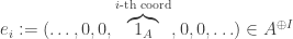
Let $I$ be any set. The free A-module on I is a direct sum of copies of A, indexed by $i\in I$ :

$A^{\oplus I} := \oplus_{i\in I} A.$

More generally, an A-module M is free if $M \cong A^{\oplus I}$ for some I. Note that M is finite free if we can pick I to be finite.

Exercise A

Prove that if A is a non-trivial ring and $A^n \cong A^m$ , then $n = m$ . [Hint: pick a maximal ideal of A; reduce this to a statement in linear algebra.]

For each $i\in I$ , let

$e_i := ( \ldots, 0, 0, \overbrace{1_A}^{i\text{-th coord}}, 0, 0, \ldots)\in A^{\oplus I}$

which takes zeros at all entries except i, where it takes $1_A$ .

Why do we use the direct sum and not the product? Well, the direct sum allows us to have the following nice properties. Following the case of linear algebra, we define:

Definition.

Let M be an A-module. A collection of elements $(m_i)_{i\in I}$ of M is said to be linearly independent over A, if for any distinct $i_1, \ldots, i_n \in I$ ,

$a_1, \ldots, a_n \in A, \ a_1 m_{i_1} + a_2 m_{i_2} + \ldots + a_n m_{i_n} = 0 \implies a_1 = a_2 = \ldots = a_n.$

If $(m_i)$ is linearly independent and generates the whole module, we call it a basis of M.

The following result comes at no surprise.

Proposition 1.

The $(e_i)$ form a basis of $A^{\oplus I}$ , called the standard basis.

M is free if and only if it has a basis indexed by I.

Proof

Easy exercise. ♦

The free module also satisfies the following universal property.

Universal Property of Free Module.

Let M be an A-module, and $\nu : I \to M$ be a set of elements in M, indexed by I; we write $m_i := \nu(i) \in M$ . Then there is a unique A-linear map

$\psi : A^{\oplus I} \to M, \quad \psi(e_i) = m_i.$

Note

In other words, we have a bijection of sets:

$\begin{aligned} \mathrm{hom}_{A\text{-}\mathbf{Mod}}(A^{\oplus I}, M) &\stackrel \cong\to \mathrm{hom}_{\mathbf{Set}}(I, M), \\ \psi &\mapsto (i \mapsto \psi(e_i)).\end{aligned}$

Exercise B

Prove the universal property.
Prove that $\psi$ is surjective if and only if the $(m_i)_{i\in I}$ generate M.

This universal property is a special case of adjoint functors in category theory, which we will see later.

blue-lin

Projective Modules

One can imagine projective modules as a generalization of free modules. Geometrically, if we think of modules over a coordinate ring $k[V]$ as vector bundles over V, then projective modules correspond to locally trivial bundles. To get acquainted with this concept, first we give the abstract definition before going through its implications.

Recall that for any A-module M, the functor $\mathrm{Hom}_A(M, -)$ is left-exact.

Definition.

The module M is said to be projective if $\mathrm{Hom}_A(M, -)$ is exact.

Thus, M is projective if and only if: for any surjective $f:N_1 \to N_2$ , the map $f_* : \mathrm{Hom}_A(M, N_1) \to \mathrm{Hom}_A(M, N_2)$ is surjective. Equivalently, any $g : M\to N_2$ lifts to some $h : M\to N_1$ such that $f\circ h = g$ :

projective_module_cd

Note

We only demand existence, not uniqueness, of h, i.e. this is not a universal property.

Lemma 1.

A free module is projective.

Proof

Without loss of generality let $M = A^{\oplus I}$ and $g : M \to N_2$ be an A-linear map. Let $n_i' = g(e_i) \in N_2$ , where $e_i \in M$ are elements of the standard basis. Since $f$ is surjective, for each $i\in I$ there exists $n_i \in N_1$ such that $f(n_i) = n_i'$ . By the universal property of the free module, there is a unique $h:M\to N_1$ which maps $e_i\mapsto n_i$ for each $i\in I$ . Then $(f\circ h)(e_i) = f(n_i) = n_i' = g(e_i)$ . Hence $f\circ h = g$ . ♦

blue-lin

Splitting Lemma

Recall that for a submodule $N\subseteq M$ we do not have $M \cong N \oplus (M/N)$ in general. However, suppose we can find another $P\subseteq M$ such that:

$N + P = M, \quad N \cap P = 0,$

then we get an isomorphism $N \oplus P \cong M$ by mapping $(x,y) \mapsto x+y$ . The proof for this is a straight-forward exercise.

Splitting Lemma.

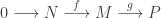
Suppose we have the following short exact sequence of A-modules.

$0 \longrightarrow N \stackrel f\longrightarrow M \stackrel g\longrightarrow P \longrightarrow 0.$

If there is an A-linear map $i : P\to M$ such that $g\circ i = 1_P$ , then $N \oplus P \cong M$ by mapping $(x,y) \mapsto f(x) + i(y)$ .

Note

For any A-modules N and P, we always have the canonical sequence

$0\longrightarrow N \stackrel f\longrightarrow N\oplus P \stackrel g \longrightarrow P \longrightarrow 0, \quad f(n) = (n, 0),\ g(n, p) = p.$

The map $i(p) = (0, p)$ then satisfies $g\circ i = 1_P$ . The splitting lemma effectively states the converse: existence of such an i means the exact sequence is isomorphic to this form.

Proof

Note that since $g\circ i$ is injective so is $i$ . Now we prove the following:

$M = f(N) + i(P), \quad f(N) \cap i(P) = 0.$

For the first claim, let $m\in M$ and $p = g(m) \in P$ . Let $m' = i(p)$ . Note that $g(m - m') = p - gi(p) = 0$ so we have $m-m' = f(n)$ for some $n\in N$ . This gives $m = f(n) + m' = f(n) + i(p)$ .

For the seecond claim, suppose $f(n) = i(p)$ for some $n\in N$ and $p\in P$ . Then $p = g(i(p)) = g(f(n)) = 0$ . ♦

Exercise C

Prove the other splitting lemma: if there is an A-linear map $j : M\to N$ such that $j\circ f = 1_N$ , then $N\oplus P \cong M$ .

blue-lin

Projective vs Free

The splitting lemma gives us the following classification of projective modules.

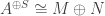
Theorem 1.

An A-module M is projective if and only if there exists an A-module N such that $M\oplus N$ is free.

Furthermore, if M is finitely generated and projective, we can pick N such that $M\oplus N$ is finite free.

Proof

Consider the equivalence in the first statement.

(⇒) Let M be projective. Pick any generating subset $S\subseteq M$ (e.g. the whole module) which gives a surjective $f: A^{\oplus S} \to M$ mapping $e_s \mapsto s$ . If M is finitely generated, we pick S to be finite. Since M is projective, the identity map $1_M : M\to M$ lifts to a map $h: M \to A^{\oplus S}$ such that $f\circ h = 1_M$ . By the splitting lemma we have $A^{\oplus S} \cong M \oplus N$ for some N. Note that this also proves the second statement.

(⇐) Suppose $M \oplus N$ is free, and hence projective. It suffices to show: if $M\oplus N$ is projective so is M. But we have a natural isomorphism

$\mathrm{Hom}_A(M\oplus N, P) \cong \mathrm{Hom}_A(M, P) \oplus \mathrm{Hom}_A(N, P)$

of functors in P. Since $M\oplus N$ is projective, the LHS is an exact functor, hence so is the RHS, and it follows that $\mathrm{Hom}_A(M, -)$ is exact. ♦

blue-lin

Examples and Consequences

At first glance, it is not entirely clear there are projective modules that are not free. Here are two examples.

Example 1

Let $B = A\times A'$ . Then $M = A\times \{0\}$ and $N=\{0\} \times A'$ are B-modules such that $M \oplus N \cong B$ . Hence M and N are projective even though they are clearly not free.

Example 2

A more interesting example occurs for $A = \mathbb Z[\sqrt{-5}]$ , a non-PID. Recall that the prime ideals

$\mathfrak p = (1+\sqrt{-5}, 2), \quad \mathfrak q = (1 - \sqrt{-5}, 2)$

are non-principal. However, they are projective because of the following.

Exercise D

Prove that we have an isomorphism of A-modules:

$A \oplus A \longrightarrow \mathfrak p \oplus \mathfrak q, \quad (x, y) \mapsto ((1+\sqrt{-5})x + 2y, ?\, x + ?\, y).$

Example 3

Let $A = \mathbb C[X, Y]/(Y^2 - X^3 + X)$ and $\mathfrak m = (X, Y)$ be a maximal ideal of A. Then $\mathfrak m$ is a projective module because of the following.

Exercise E

Prove that we have an isomorphism of A-modules

$A \oplus A \longrightarrow \mathfrak m \oplus \mathfrak m, \quad (f, g) \mapsto (X f + Y g, ?\, f + ?\, g).$

Now we discuss some consequences of the above results.

Corollary 1.

If $(M_i)$ is a collection of projective A-modules, then $\oplus_i M_i$ is projective.

Proof

For each i let $N_i$ be an A-module such that $M_i \oplus N_i$ is free. Then $(\oplus_i M_i) \oplus (\oplus_i N_i) \cong \oplus_i (M_i \oplus N_i)$ is also free. Hence $\oplus_i M_i$ is projective. ♦

Corollary 2.

If M is a projective A-module, then $S^{-1}M$ is a projective $S^{-1}A$ -module.

Proof

Indeed, if $M \oplus N \cong A^{\oplus I}$ then

$(S^{-1}M) \oplus (S^{-1}N) \cong S^{-1}(M\oplus N) \cong S^{-1}(A^{\oplus I}) \cong (S^{-1}A)^{\oplus I}$

because localization commutes with taking direct sums. Hence $S^{-1}M$ is also projective over $S^{-1}A$ . ♦

Is projective a local property then? In other words, suppose M is an A-module such that $M_{\mathfrak m}$ is projective over $A_{\mathfrak m}$ for all maximal $\mathfrak m$ , must M be projective? We will answer this in a later article (spoiler: the answer is a conditional ‘yes’).

blue-lin

Posted in Advanced Algebra | Tagged exact functors, free modules, left-exact, localization, projective modules, splitting lemma | Leave a comment

Commutative Algebra 26

Posted on April 13, 2020 by limsup

Left-Exact Functors

We saw (in theorem 1 here) that the localization functor $M \mapsto S^{-1}M$ is exact, which gave us a whole slew of nice properties, including preservation of submodules, quotient modules, finite intersection/sum, etc. However, exactness is often too much to ask for.

Throughout this article, A and B are fixed rings and $F: A\text{-}\mathbf{Mod} \to B\text{-}\mathbf{Mod}$ is a covariant additive functor.

Definition.

We say F is left-exact if it takes a short exact sequence of A-modules

$0 \longrightarrow N \stackrel f\longrightarrow M \stackrel g\longrightarrow P \longrightarrow 0$

to an exact sequence of B-modules

$0 \longrightarrow F(N) \stackrel {F(f)}\longrightarrow F(M) \stackrel {F(g)} \longrightarrow F(P).$

Immediately we can weaken the condition.

Lemma 1.

F is left-exact if and only if it takes an exact sequence of A-modules

$0 \longrightarrow N \stackrel f\longrightarrow M \stackrel g\longrightarrow P$

to an exact sequence of B-modules

$0 \longrightarrow F(N) \stackrel {F(f)}\longrightarrow F(M) \stackrel {F(g)} \longrightarrow F(P).$

Proof

(⇐) is obvious. For (⇒) given an exact $0 \to N \stackrel f\to M \stackrel g\to P$ , we extend it to an exact $0 \to N \to M \to P \to \mathrm{coker } g \to 0$ . [Recall that $\mathrm{coker } g = P/\mathrm{im } g$ is the cokernel of g.] We can split this exact sequence into short exact ones:

$\begin{aligned} 0 \to N \stackrel f\to M \to \mathrm{im } g \to 0 &\implies 0 \to F(N) \stackrel{F(f)}\to F(M) \to F(\mathrm{im } g)\\ 0 \to \mathrm{im } g \to P \to \mathrm{coker } g \to 0 &\implies 0 \to F(\mathrm{im } g) \to F(P) \to F(\mathrm{coker } g).\end{aligned}$

which gives an exact sequence $0\to F(N) \to F(M) \to F(P)$ as desired. ♦

Note

Left-exact functors are not as nice as exact ones but we still get some useful results out of them. For example, if $f : N\to M$ is injective, so is $F(f) : F(N) \to F(M)$ so for a submodule $N\subseteq M$ , we can consider $F(N)$ as a submodule of $F(M)$ .

Also, for any $f:N\to M$ , since $0\to \mathrm{ker } f \to N \to M$ is exact, applying F gives an exact $0 \to F(\mathrm{ker} f) \to F(N) \stackrel{F(f)}\to F(M)$ and thus $F(\mathrm{ker} f) = \mathrm{ker } F(f)$ .

blue-lin

Hom Functors Are Left-Exact

The main result we wish to show is

Proposition 1.

For any A-module M, the functor $\mathrm{Hom}_A(M, -)$ is a left-exact functor.

Proof

Take the exact sequence $0 \to N_1 \stackrel f\to N_2 \stackrel g\to N_3$ . We need to show that

$0 \longrightarrow \mathrm{Hom}_A(M, N_1) \stackrel {f_*}\longrightarrow \mathrm{Hom}_A(M, N_2) \stackrel{g_*}\longrightarrow \mathrm{Hom}_A(M, N_3)$

is exact. It is easy to show $f_*$ is injective (easy exercise). Next, we have

$g_*\circ f_* = (g\circ f)_* = 0 \implies \mathrm{im } f_* \subseteq \mathrm{ker } g_*.$

Conversely suppose $h:M\to N_2$ satisfies $g_*(h) = g\circ h = 0$ . Then $\mathrm{im } h \subseteq \mathrm{ker } g = \mathrm{im } f$ . Since f is injective it follows that for each $m\in M$ , we have $h(m) = f(x)$ for a unique $x\in N_1$ . This map $h' : M \to N_1, m\mapsto x$ is clearly A-linear so $h = f\circ h' = f_*(h')$ . ♦

Here is one application of this result.

Corollary 1.

Let $a\in A$ ; for each A-module, let $M[a] = \{m \in M : am = 0\}$ . Then

$0 \longrightarrow N \stackrel f \longrightarrow M \stackrel g \longrightarrow P \text{ exact } \implies 0 \longrightarrow N[a] \stackrel f\longrightarrow M[a] \stackrel g \longrightarrow P[a] \text{ exact.}$

Proof

Indeed the functor $M\mapsto M[a]$ is naturally isomorphic to $\mathrm{Hom}_A(A/(a), -)$ . Now apply the above. ♦

Exercise A

Find a surjective $M\to P$ for which $M[a] \to P[a]$ is not surjective. This shows that the functor $\mathrm{Hom}_A(M, -)$ is not exact in general.

blue-lin

Converse Statement

Next we have the following converse.

Proposition 2.

Suppose $f:N_1 \to N_2$ and $g:N_2\to N_3$ are A-linear maps such that for any A-module M,

$0\longrightarrow \mathrm{Hom}_A(M, N_1) \stackrel {f_*} \longrightarrow \mathrm{Hom}_A(M, N_2) \stackrel {g_*} \longrightarrow \mathrm{Hom}_A(M, N_3)$

is exact. Then $0 \to N_1 \stackrel f \to N_2 \stackrel g \to N_3$ is exact.

Proof

First we show f is injective. Let $M =\mathrm{ker } f$ so that $0 \to M \to N_1 \stackrel {f} \to N_2$ is exact. By left-exactness of Hom we have an exact:

$0 \to {\mathrm{Hom}_A(M, M)} \to \mathrm{Hom}_A(M, N_1) \stackrel {f_*} \to \mathrm{Hom}_A(M, N_2)$ .

Since $f_*$ is injective, $\mathrm{Hom}_A(M, M) = 0$ and in particular $1_M = 0\implies M=0$ .

Next we show $g\circ f = 0$ . Setting $M = N_1$ gives:

$0 = g_* f_* (\mathrm{Hom}_A(N_1, N_1)) = (g\circ f)_*(\mathrm{Hom}_A(N_1, N_1))$

so $g\circ f = (g\circ f)_* (1_{N_1}) = 0.$ This gives $\mathrm{im } f \subseteq \mathrm{ker } g$ .

Finally we set $M = \mathrm{ker } g$ . The following sequence:

$0\longrightarrow \mathrm{Hom}_A(M, N_1) \stackrel {f_*} \longrightarrow \mathrm{Hom}_A(M, N_2) \stackrel {g_*} \longrightarrow \mathrm{Hom}_A(M, N_3)$

is exact. The inclusion $i : M\hookrightarrow N_2$ gives $g_*(i) = g\circ i = 0$ and so $i = f_*(j) = f\circ j$ for some $j : M \to N_1$ . Then $M = \mathrm{im } i \subseteq \mathrm{im } f$ . ♦

blue-lin

Another Left-Exactness

Now suppose $F: A\text{-}\mathbf{Mod} \to B\text{-}\mathbf{Mod}$ is a contravariant additive functor.

Definition.

We say F is left-exact if it takes a short exact sequence of A-modules

$0 \longrightarrow N \stackrel f\longrightarrow M \stackrel g\longrightarrow P \longrightarrow 0$

to an exact sequence of B-modules

$0 \longrightarrow F(P) \stackrel {F(g)}\longrightarrow F(M) \stackrel {F(f)} \longrightarrow F(N).$

Again we have:

Lemma 2.

F is left-exact if and only if it takes an exact sequence of A-modules

$N \stackrel f\longrightarrow M \stackrel g\longrightarrow P \longrightarrow 0$

to an exact sequence of B-modules

$0 \longrightarrow F(P) \stackrel {F(g)}\longrightarrow F(M) \stackrel {F(f)} \longrightarrow F(N).$

Proof

Exercise. ♦

Now we show, as before:

Proposition 3.

For any A-module M, the functor $\mathrm{Hom}_A(-, M)$ is a left-exact functor.

Proof

Take the exact sequence $N_1 \stackrel f\to N_2 \stackrel g\to N_3 \to 0$ . We need to show that

$0 \longrightarrow \mathrm{Hom}_A(N_3, M) \stackrel {g^*}\longrightarrow \mathrm{Hom}_A(N_2, M) \stackrel{f^*}\longrightarrow \mathrm{Hom}_A(M, N_1)$

is exact for any A-module M. Injectivity of $g^*$ is obvious. Also $f^* \circ g^* = (g\circ f)^* = 0$ so $\mathrm{im } g^* \subseteq \mathrm{ker } f^*$ .

It remains to show $\mathrm{ker } f^* \subseteq \mathrm{im } g^*$ . Pick $h: N_2 \to M$ such that $f^*(h) = h\circ f = 0$ so that $\mathrm{ker } g = \mathrm{im } f \subseteq \mathrm{ker } h$ . Hence h factors through $N_2 / \mathrm{ker } g \to M$ . Since $N_2 / \mathrm{ker } g \cong N_3$ , we have $h = h'\circ g = g^*(h'')$ for some $h' : N_3 \to M$ . ♦

blue-lin

Another Converse Statement

Finally, the reader should expect the following.

Proposition 4.

Suppose $f:N_1 \to N_2$ and $g:N_2\to N_3$ are A-linear maps such that for any A-module M,

$0\longrightarrow \mathrm{Hom}_A(N_3, M) \stackrel {g^*} \longrightarrow \mathrm{Hom}_A(N_2, M) \stackrel {f^*} \longrightarrow \mathrm{Hom}_A(N_1, M)$

is exact. Then $N_1 \stackrel f \to N_2 \stackrel g \to N_3 \to 0$ is exact.

Proof

We leave it as an exercise to show: g is surjective, $g\circ f = 0$ .

It remains to show $\mathrm{ker } g \subseteq \mathrm{im } f$ ; let $M = \mathrm{coker } f$ and take the exact sequence

$0\longrightarrow \mathrm{Hom}_A(N_3, M) \stackrel {g^*} \longrightarrow \mathrm{Hom}_A(N_2, M) \stackrel {f^*} \longrightarrow \mathrm{Hom}_A(N_1, M)$

If $\pi : N_2 \to M$ is the canonical map, $f^*(\pi) = \pi\circ f = 0$ so we have $\pi = g^*(j) = j\circ g$ for some $j : N_3 \to M$ . Thus $\mathrm{ker } g \subseteq \mathrm{ker } \pi = \mathrm{im } f$ . ♦

As an application, let us prove the following.

Corollary 2.

Let $\mathfrak a \subseteq A$ be an ideal. If $N \to M \to P \to 0$ is an exact sequence of A-modules, then we get an exact sequence of $(A/\mathfrak a)$ -modules:

$N/\mathfrak a N \longrightarrow M/\mathfrak a M \longrightarrow P/\mathfrak a P \longrightarrow 0.$

Proof

Let $B = A/\mathfrak a$ . It suffices to show that for any B-module Q, the sequence

$0 \longrightarrow \mathrm{Hom}_B(P/\mathfrak a P, Q) \longrightarrow \mathrm{Hom}_B(M/\mathfrak a M, Q) \longrightarrow \mathrm{Hom}_B(N/\mathfrak a N, Q)$

is exact. But since $M\mapsto M/\mathfrak a M$ gives the B-module induced from M, the above sequence is naturally isomorphic to:

$0 \longrightarrow \mathrm{Hom}_A(P, Q) \longrightarrow \mathrm{Hom}_A (M, Q) \longrightarrow \mathrm{Hom}_A(N, Q)$

which we know is exact because the Hom functor is left-exact. ♦

This leads to the following definition.

Definition.

Suppose $F: A\text{-}\mathbf{Mod} \to B\text{-}\mathbf{Mod}$ is a covariant additive functor. We say F is right-exact if it takes a short exact sequence of A-modules

$0 \longrightarrow N \stackrel f\longrightarrow M \stackrel g\longrightarrow P \longrightarrow 0$

to an exact sequence of B-modules

$F(N) \stackrel {F(f)}\longrightarrow F(M) \stackrel {F(g)} \longrightarrow F(P) \longrightarrow 0.$

Exercise B

Prove that F is right-exact if and only if it takes an exact sequence of A-modules $N \to M \to P \to 0$ to an exact sequence of B-modules $F(N) \to F(M) \to F(P) \to 0.$

Thus, we have shown that the functor

$A\text{-}\mathbf{Mod} \longrightarrow (A/\mathfrak a)\text{-}\mathbf{Mod}, \quad M \mapsto M/\mathfrak aM$

is right-exact. This will be generalized in future chapters.

Exercise C

Prove that the functor $M\mapsto M/\mathfrak a M$ is not exact in general.
Use a direct proof to show $M\mapsto M/\mathfrak a M$ is right-exact.

In summary, we have covered the following concepts:

exact_functor_types

blue-lin

Posted in Advanced Algebra | Tagged additive functors, hom functor, induced modules, left-exact, right-exact | Leave a comment

Commutative Algebra 25

Posted on April 12, 2020 by limsup

Arbitrary Collection of Modules

Finally, we consider the case where we have potentially infinitely many modules.

Proposition 1.

For a collection of A-modules $(M_i)_{i\in I}$ , we have

$S^{-1}(\oplus_i M_i) \cong \oplus_i (S^{-1} M_i).$

Proof

First claim: we will show that the LHS satisfies the universal property for direct sums. Now for any $S^{-1}A$ -module N, we have:

$\begin{aligned} \mathrm{Hom}_{S^{-1}A}(\oplus_i (S^{-1}M_i), N)&\cong \prod_{i\in I}\mathrm{Hom}_{S^{-1}A} (S^{-1}M_i, N) \\ &\cong \prod_{i\in I} \mathrm{Hom}_A(M_i, N) \\ &\cong \mathrm{Hom}_A(\oplus_i M_i, N) \\ &\cong \mathrm{Hom}_{S^{-1}A}(S^{-1}(\oplus_i M_i), N).\end{aligned}$

The first correspondence follows from the universal property of direct sums.
The second follows from the universal property of localization $S^{-1}M_i$ .
The third follows from the universal property of direct sums.
The last follows from the universal property of localization $S^{-1}(\oplus_i M_i)$ .

This is a natural isomorphism, with both sides functorial in N. Now apply the following to get an isomorphism of A-modules

$S^{-1}(\oplus_i M_i) \cong \oplus_i (S^{-1} M_i).$ ♦

Exercise A

Prove the following corollary of Yoneda lemma: if $A, B \in \mathcal C$ are objects such that there is a natural isomorphism

$\mathrm{hom}_{\mathcal C}(A, -) \cong \mathrm{hom}_{\mathcal C}(B, -)$

then $A \cong B$ in $\mathcal C$ .

warning In general, localization does not commute with direct products:

$S^{-1} (\prod_i M_i) \ne \prod_i S^{-1} M_i.$

To be specific, the projection maps $\prod_i M_i \to M_j$ for indices j induce $S^{-1}(\prod_i M_i) \to S^{-1}M_j$ , and by the universal property of products

$S^{-1}(\prod_i M_i) \longrightarrow \prod_i (S^{-1} M_i)$

which is not an isomorphism in general. For example, we can set $A = \mathbb Z$ and $S = \mathbb Z - \{0\}$ . If $M_1 = M_2 = \ldots = \mathbb Z$ , then $(1, \frac 1 2, \frac 1 3, \ldots)$ in the RHS is not in the image of the map.

Exercise B

1. Find A-submodules $N_i \subseteq M$ such that $S^{-1}(\cap_i N_i) \ne \cap_i S^{-1} N_i$ as submodules of $S^{-1}M$ .

2. Prove that for a collection of A-submodules $(N_i)_{i\in I}$ of M, we have

$S^{-1}(\sum_i N_i) = \sum_i S^{-1} N_i$ ,

as submodules of $S^{-1}M$ . [Hint: use a straightforward proof.]

blue-lin

Local Properties

Another important property we wish to emphasize is locality. As a motivation suppose V is an irreducible k-variety (k algebraically closed) with $A = k[V]$ , which is a domain.

Let $\phi : V\to k$ be a function such that for each $P\in V$ , $\phi$ is regular at P.

Thus V is a union of open subsets $U_i$ such that each restriction $\phi |_{U_i}$ can be locally written as $P\mapsto \frac {f(P)}{g(P)}$ where $f,g \in k[V]$ and $g(P) \ne 0$ for all $P\in U_i$ . We claim that this implies $\phi\in k[V]$ , or to be specific, there exists $f\in k[V]$ such that $f(P) = \phi(P)$ for all $P\in V$ .

Indeed, the preceding condition says $\phi \in k[V]_{\mathfrak m_P}$ for all $P\in V$ , and since all maximal ideals of $k[V]$ are of the form $\mathfrak m_P$ , we only need to show:

Proposition 2.

For any integral domain A, $A = \cap_{\mathfrak m \text{ maximal }} A_{\mathfrak m}$ , where intersection occurs in the field of fractions $\mathrm{Frac}(A)$ of A.

Proof

(⊆) is obvious. For (⊇), suppose $f\in K$ lies in all $A_{\mathfrak m}$ . Let $\mathfrak a = \{a \in A : af \in A\}$ . Note that $\mathfrak a$ is an ideal of A, since if $af, a'f \in A$ then $(a+a')f = af+a'f \in A$ , and if $af\in A$ then for any $b\in A$ we have $baf \in A$ as well.

If $\mathfrak a \ne (1)$ , then $\mathfrak a\subseteq \mathfrak m$ for some maximal ideal $\mathfrak m \subset A$ . But $f \in A_{\mathfrak m}$ so for some $s \in A-\mathfrak m$ we have $sf\in A$ . Thus $s \in \mathfrak a - \mathfrak m$ , a contradiction. ♦

When we look at $A=\mathbb Z$ , this becomes quite obvious: when p is prime, $\mathbb Z_{(p)}$ is the ring of $\frac a b \in \mathbb Q$ where a, b are integers and b is not a multiple of p. Hence if $\frac a b\in \mathbb Q$ (reduced) lies in all $\mathbb Z_{(p)}$ it just means b is not divisible by any prime, so $b = \pm 1$ .

blue-lin

More Local Properties

In all the following results, $\mathfrak m$ denotes a maximal ideal of A.

Proposition 3.

Let M be an A-module. Then $M=0$ if and only if $M_{\mathfrak m} = 0$ for all $\mathfrak m$ .

Proof

(⇒) is obvious. For (⇐) fix $m\in M$ and let $\mathfrak a = \{a \in A : am = 0\}$ . It is easy to show that this is an ideal of A. Now for any maximal ideal $\mathfrak m$ , since $\frac m 1 \in M_{\mathfrak m}$ is zero there exists $s\in A-\mathfrak m$ such that $sm = 0$ . Thus $s \in \mathfrak a - \mathfrak m$ . Since $\mathfrak a$ is an ideal not contained in any maximal ideal, it is (1), i.e. $1\in \mathfrak a$ so $m=0$ . ♦

Note

The ideal $\mathfrak a$ above is called the annihilator of m; we will have more to say about it later.

Proposition 4.

Let $f:M\to N$ be a homomorphism of A-modules. Then $f$ is zero if and only if $f_{\mathfrak m} : M_{\mathfrak m} \to N_{\mathfrak m}$ is zero for all $\mathfrak m$ .

Proof

(⇐) : for each $\mathfrak m$ we have $(\mathrm{im} f)_{\mathfrak m} = \mathrm{im} f_{\mathfrak m} = 0$ since $f_{\mathfrak m} = 0$ . Thus by proposition 3, $\mathrm{im} f = 0$ and we have $f=0$ . ♦

Corollary 1.

Let $f, g:M\to N$ be homomorphisms of A-modules. Then $f=g$ if and only if $f_{\mathfrak m} = g_{\mathfrak m}$ for all $\mathfrak m$ .

Proof.

Apply proposition 4 to $f-g$ . ♦

Proposition 5.

Let $N\stackrel f\to M \stackrel g\to P$ be A-linear maps. The sequence is exact if and only if

$N_{\mathfrak m} \stackrel {f_{\mathfrak m}} \longrightarrow M_{\mathfrak m} \stackrel {g_{\mathfrak m}} \longrightarrow P_{\mathfrak m}$

is exact for each $\mathfrak m$ .

Proof

(⇒) We saw in theorem 1 here that localization is an exact functor.

(⇐) First we show that $\mathrm{im} f \subseteq \mathrm{ker} g$ , or equivalently $g\circ f = 0$ . But $(g\circ f)_{\mathfrak m} = g_{\mathfrak m} \circ f_{\mathfrak m} = 0$ for each $\mathfrak m$ so $g\circ f = 0$ .

For the reverse inclusion, consider the module $(\mathrm{ker} g) / (\mathrm{im} f)$ . We have

$((\mathrm{ker} g) / (\mathrm{im} f))_{\mathfrak m} \cong (\mathrm{ker} g)_{\mathfrak m} / (\mathrm{im} f)_{\mathfrak m} \cong (\mathrm{ker} g_{\mathfrak m}) / (\mathrm{im} f_{\mathfrak m}).$

Since this is zero for all $\mathfrak m$ , we have $\mathrm{ker} g = \mathrm{im} f$ . ♦

Corollary 2.

An A-linear map $f: M\to N$ is injective (resp. surjective) if and only if $f_{\mathfrak m} : M_{\mathfrak m} \to N_{\mathfrak m}$ is injective (resp. surjective) for each $\mathfrak m$ .

Proof

Apply proposition 5 to $0\to M \stackrel f\to N$ and $M\stackrel f\to N \to 0$ respectively. ♦

Note

As a general statement, we say the above properties are local. Philosophically, this means in order to check a certain property, it suffices to check at each maximal ideal so we can restrict ourselves to the case where the base ring is local. With Nakayama’s lemma, we will see that finitely generated modules over local rings are quite well-behaved.

Geometrically, this says we only need to look at each point of the variety to check the property. For example, if we interpret modules over the coordinate ring as vector bundles over the variety, then locality says: a bundle map $E \to F$ is injective if and only if $E_P \to F_P$ is injective at every point P.

Exercise C

Recall that the localization of a reduced ring is reduced, and that of an integral domain is an integral domain. Decide if each of the following is true and justify your answer.

If $A_{\mathfrak m}$ is reduced for all $\mathfrak m$ , then so is A.
If $A_{\mathfrak m}$ is an integral domain for all $\mathfrak m$ , then so is A.

blue-lin

Posted in Advanced Algebra | Tagged direct products, direct sums, exact sequences, local properties, local rings, localization | Leave a comment

Commutative Algebra 24

Posted on April 11, 2020 by limsup

Quotient vs Localization

Taking the quotient $A \mapsto A/\mathfrak a$ and localization $A \mapsto S^{-1}A$ are two sides of the same coin when we look at $\mathrm{Spec A}$ .

Quotient removes the “small” prime ideals in $\mathrm{Spec A}$ – it only keeps the prime ideals containing $\mathfrak a$ .
Localization removes the “large” prime ideals in $\mathrm{Spec A}$ – it only keeps prime ideals disjoint from S.

It turns out these two operations commute.

Proposition 1.

Let $\mathfrak a\subseteq A$ be an ideal and $S\subseteq A$ a multiplicative subset.

Let $T = \{\overline s \in A/\mathfrak a : s \in S\}$ , a multiplicative subset of $A/\mathfrak a$ .

Let $\mathfrak b = \mathfrak a (S^{-1}A)$ , an ideal of $S^{-1}A$ .

Then we have an isomorphism

$(S^{-1}A) / \mathfrak b \stackrel\cong\longrightarrow T^{-1}(A/\mathfrak a), \quad \overline{a/s} \leftrightarrow \overline a/\overline s$ .

Proof

We will use the universal properties here.

The canonical homomorphism $\phi : A\to S^{-1}A$ gives us $\phi (\mathfrak a) \subseteq \mathfrak a (S^{-1}A) = \mathfrak b$ . Thus we get a ring homomorphism $A/\mathfrak a \to (S^{-1}A)/\mathfrak b$ which takes $\overline a \mapsto \overline {a/1}$ . This map takes every element of $T$ to a unit so it factors through $A/\mathfrak a \to T^{-1}(A/\mathfrak a) \to (S^{-1}A)/\mathfrak b$ . The latter map takes $\overline a / \overline 1 \mapsto \overline {a/1}$ and thus $\overline a / \overline s \mapsto \overline {a/s}$ .

The reverse map is left as an exercise. [Hint: start with $A \to A/\mathfrak a \to T^{-1}(A/\mathfrak a)$ .] ♦

Definition.

Let $\mathfrak p \in \mathrm{Spec} A$ be a prime ideal. The residue field $k(\mathfrak p)$ is defined equivalently as:

the field of fractions of $A/\mathfrak p$ , or

the quotient of local ring $A_{\mathfrak p}$ by its unique maximal ideal.

Thanks to proposition 1, the definition is sensible (let $\mathfrak a = \mathfrak p$ and $S = A - \mathfrak p$ ).

Question to Ponder

If $A = k[V]$ is the coordinate ring of a variety over algebraically closed k, what do elements of $k(\mathfrak p)$ correspond to?

blue-lin

Localization of Modules

Let M be an A-module and S a multiplicative subset of A.

Proposition 2.

The localized module $S^{-1}M$ is defined as $m/s$ with $m\in M$ and $s\in S$ under the equivalence

$m/s = m'/s' \iff (\exists t\in S, \ t(s'm - sm') = 0).$

Now $S^{-1}M$ becomes an $S^{-1}A$ -module via:

$\frac m s, \frac {m'}{s'} \in S^{-1}M, \ \frac a t\in S^{-1}A \implies \begin{cases} \frac m s + \frac {m'}{s'} = \frac{s'm + sm'}{ss'}, \\ \frac a t \cdot \frac m s = \frac{am}{ts}.\end{cases}$

Proof

Easy exercise (but tedious!). ♦

Proposition 3.

The $S^{-1}A$ -module $S^{-1}M$ satisfies the following universal property. We have the pair

$(S^{-1}M, \phi : M \to S^{-1}M)$

where $S^{-1}M$ is an $S^{-1}A$ -module, $\phi(m) := \frac m 1$ is A-linear, such that for any pair

$(N, \psi : M\to N)$

where $N$ is an $S^{-1}A$ -module and $\psi$ is A-linear, there is a unique $S^{-1}A$ -linear map $f : S^{-1}M \to N$ such that $f\circ \phi = \psi$ .

Note

Universal property thus says we get a bijection for any $S^{-1}A$ -module N:

$\begin{aligned} \mathrm{Hom}_{S^{-1}A}(S^{-1}M, N) \stackrel \cong \to &\mathrm{Hom}_A(M, N), \\ f \mapsto &f\circ \phi. \end{aligned}$

Proof

Existence: given $(N, \psi:M \to N)$ , we define $f:S^{-1}M \to N$ by $\frac m s \mapsto \frac 1 s \cdot \psi(m)$ . It is well-defined: if $\frac m s = \frac {m'}{s'}$ then $t(s'm) = t(sm')$ for some $t\in S$ , and so $ts'\cdot \psi(m) = ts\cdot \psi(m')$ , which gives $\frac 1 s \cdot\psi(m) = \frac 1 {s'}\cdot \psi(m')$ since t acts bijectively on N. It is easy to check f is $S^{-1}A$ -linear and $f\circ \phi(m) = f(\frac m 1) = \psi(m)$ .

Uniqueness: suppose $f : S^{-1}M \to N$ is $S^{-1}A$ -linear and $f(\frac m 1) = \psi(m)$ for every $m \in M$ . Then

$\frac m s \in S^{-1}M \implies \psi(m) = f(\frac m 1) = f(\frac s 1\cdot\frac m s) = \frac s 1 f(\frac m s)$

so $f(\frac m s) =\frac 1 s \cdot \psi(m)$ . ♦

blue-lin

Functoriality

Definition.

Suppose $f:M\to N$ is an A-linear map. We have an $S^{-1}A$ -linear map

$S^{-1}f : S^{-1}M \longrightarrow S^{-1}N, \quad \frac m s \mapsto \frac {f(m)}s.$

Proof

Let us check the map is well-defined. If $\frac m s = \frac {m'}{s'}$ then $t(s'm - sm') = 0$ for some $t\in S$ . Applying f gives $t(s'\cdot f(m) - s\cdot f(m')) = 0$ and hence $\frac{f(m)}s = \frac{f(m')}{s'}$ . Linearity is an easy exercise. ♦

Clearly $S^{-1}(1_M) = 1_{S^{-1}M}$ and $S^{-1}(g\circ f) = (S^{-1}g) \circ (S^{-1}f)$ for any $f: N\to M$ and $g:M\to P$ . Thus localization gives a functor

localization_functor

Furthermore, the functor is A-linear, i.e. for A-modules M and N,

$a\in A,\ f, g : M\to N \implies \begin{cases} &S^{-1}f + S^{-1}g = S^{-1}(f+g), \\ &S^{-1}(af) = \frac a 1 S^{-1} f \end{cases}$

In particular, it is additive.

Generalization

One can generalize the localization functor.

Definition.

Let $B$ be an $A$ -algebra and $M$ an $A$ -module. The B-module induced from M comprises of a pair

$(M^B, \phi : M\to M^B)$

where $M^B$ is a B-module, $\phi$ is A-linear, such that for any pair

$(N, \psi : M\to N)$

where $N$ is a B-module and $\psi$ is A-linear, there is a unique B-linear $f : M^B \to N$ such that $f\circ \phi =\psi$ .

Note

Again universal property says the following is a bijection for any B-module N:

$\begin{aligned} \mathrm{Hom}_B(M^B, N) \stackrel \cong \to &\mathrm{Hom}_A(M, N), \\ f \mapsto &f\circ \phi. \end{aligned}$

Exercise A

1. Prove uniqueneess of f in the above example.

2. Prove that for an ideal $\mathfrak a \subseteq A$ and $B = A/\mathfrak a$ , the B-module induced from M is $M^B = M/\mathfrak a M$ . This explains what we meant when we said the construction is canonical.

Question to Ponder

Does $M\mapsto M^B$ give an additive functor from the category of A-modules to the category of B-modules? Can all the necessary constructions and properties be deduced just from the universal property of induced modules?

In later articles, we will give an explicit construction of the induced module.

blue-lin

Exactness

This result is of paramount importance.

Theorem 1.

The localization functor is exact, i.e. if $N\stackrel f\to M \stackrel g \to P$ is exact, so is

$S^{-1}N \stackrel {S^{-1}f}\longrightarrow S^{-1}M \stackrel{S^{-1}g} \longrightarrow S^{-1}P$ .

Proof

For any $\frac n s \in S^{-1}N$ we have $(S^{-1}g) (S^{-1}f)(\frac n s) = (S^{-1}g) (\frac {f(n)}s) = \frac{gf(n)}s = 0$ and so $\mathrm{im} (S^{-1}f) \subseteq \mathrm{ker} (S^{-1}g)$ .

Conversely suppose $(S^{-1}g)(\frac m s) = \frac{g(m)}s = 0$ . Then there exists $t\in S$ , $t\cdot g(m) = 0$ so $g(tm) = 0$ and $tm \in \mathrm{ker} g = \mathrm{im} f$ . We thus have $tm = f(n)$ for some $n\in N$ which gives us $\frac m s = \frac{f(n)}{st} = (S^{-1}f)(\frac n {st})$ . ♦

Now all the properties we proved about exact additive functors can be ported over here.

1. If $f : N\to M$ is injective, so is $S^{-1} f : S^{-1}N \to S^{-1}M$ . Hence for A-submodule $N\subseteq M$ we may regard $S^{-1}N$ as an $S^{-1}A$ -submodule of $S^{-1}M$ .

2. If $g : M\to P$ is surjective, so is $S^{-1} g : S^{-1}M \to S^{-1}P$ .

3. For A-submodule $N\subseteq M$ , we have $S^{-1}(M/N) \cong (S^{-1}M)/(S^{-1}N)$ .

4. For an A-linear map $f:N\to M$ we have

$F(\mathrm{ker} f) = \mathrm{ker} F(f), \quad F(\mathrm{coker} f) = \mathrm{coker} F(f), \quad F(\mathrm{im} f) = \mathrm{im} F(f).$

5. For A-submodules $N_1, N_2\subseteq M$ we have, as submodules of $S^{-1}M$ ,

$S^{-1}(N_1 + N_2) = (S^{-1}N_1) + (S^{-1}N_2), \quad S^{-1}(N_1 \cap N_2) = (S^{-1}N_1) \cap (S^{-1}N_2).$

Exercise B

Prove that for an ideal $\mathfrak a\subseteq A$ ,

the localized module $S^{-1}\mathfrak a$ is the ideal $\mathfrak a(S^{-1}A)$ we saw earlier,
for any A-module M we have $(S^{-1}\mathfrak a)(S^{-1} M) = S^{-1}(\mathfrak a M)$ as $S^{-1}A$ -submodules of $S^{-1}M$ .

blue-lin

Posted in Advanced Algebra | Tagged algebras, exact functors, induced modules, localization, universal properties | 2 Comments

Commutative Algebra 23

Posted on April 10, 2020 by limsup

Localization and Spectrum

Recall that the ideals of $S^{-1}A$ correspond to a subset of the ideals of A. If we restrict ourselves to prime ideals, we get the following nice bijection.

prime_ideals_of_localization

Theorem 1.

The above gives a bijection between

$\{ \mathfrak p \in \mathrm{Spec} A : \mathfrak p \cap S = \emptyset \} \leftrightarrow \mathrm{Spec} (S^{-1}A)$

Useful trick

If $\mathfrak a \subseteq A$ is an ideal, then $\frac a s \in \mathfrak a (S^{-1}A)$ implies $s'a \in \mathfrak a$ for some $s'\in S$ . Proof: exercise.

Proof

First we show $\mathfrak q = \mathfrak p (S^{-1}A)$ is prime in $S^{-1}A$ . Suppose $a,b \in A$ , $s, t\in S$ satisfy $\frac a s \frac b t \in \mathfrak q$ . Then by the above trick, there exists $s'\in S$ such that $s'ab \in \mathfrak p$ . But $\mathfrak p \cap S = \emptyset \implies s'\not\in \mathfrak p$ so either $a\in \mathfrak p$ or $b \in \mathfrak p$ and hence $\frac a s \in \mathfrak q$ or $\frac b t \in \mathfrak q$ .

Note that $\mathfrak q$ is not the whole ring since if it contains 1, then for some $a\in\mathfrak p$ , $s\in S$ ,

$\frac a s = \frac 1 1 \implies \exists t \in S, t(s-a) = 0 \implies ts = ta \in S \cap \mathfrak p,$ a contradiction.

Continuing the previous paragraph, it remains to show $\mathfrak p = \mathfrak q \cap A$ .

(⊆) Suppose $a\in \mathfrak p$ so $\frac a 1 \in \mathfrak p (S^{-1}A) = \mathfrak q$ . Thus $a \in \mathfrak q \cap A$ .

(⊇) Suppose $a \in \mathfrak q \cap A$ so that $\frac a 1 \in \mathfrak q = \mathfrak p (S^{-1}A)$ . Then $sa \in \mathfrak p$ for some $s\in S$ . Since $s\not\in \mathfrak p$ we have $a\in \mathfrak p$ . ♦

Proposition 1.

The above map identifies $\mathrm{Spec} S^{-1}A$ as a subspace of $\mathrm{Spec} A$ .

Proof

Let $\phi : A\to S^{-1}A, a\mapsto \frac a 1$ . Then $\phi^* : \mathrm{Spec} S^{-1}A \to \mathrm{Spec} A$ is injective and continuous. On the other hand, suppose $V(\mathfrak b)$ is a closed subset of $\mathrm{Spec} S^{-1}A$ for an ideal $\mathfrak b \subseteq S^{-1}A$ . Let $\mathfrak a = \mathfrak b \cap A$ , an ideal of A. It remains to show $V(\mathfrak b) = (\phi^*)^{-1} (V(\mathfrak a))$ .

(⊆) Suppose $\mathfrak q \supseteq \mathfrak b$ , a prime ideal of $S^{-1}A$ . Then $\phi^*(\mathfrak q) = \mathfrak q \cap A \supseteq \mathfrak b \cap A = \mathfrak a$ so $\phi^*(\mathfrak q) \in V(\mathfrak a)$ .

(⊇) Suppose $\mathfrak p := \phi^*(\mathfrak q) = \mathfrak q \cap A$ is a prime of A containing $\mathfrak a$ . By theorem 1, $\mathfrak q = \mathfrak p (S^{-1}A) \supseteq \mathfrak a (S^{-1}A) =\mathfrak b$ from the previous article. ♦

Philosophically, localization removes prime ideals which are “too big”.

blue-lin

Basic Open Sets

Let $f\in A$ . By the above result, $\mathrm{Spec} A_f$ is identified with the subspace $\{ \mathfrak p \in \mathrm{Spec} A : \mathfrak p \not\ni f\}$ . But this is exactly the basic open set $D(f)$ . Hence,

$\mathrm{Spec} A_f \cong D(f) \subseteq \mathrm{Spec} A$

as a homeomorphism.

Geometric Example

Let $A = k[V]$ be the coordinate ring of variety V over an algebraically closed field k. Pick $f\in A$ and let $B = A_f \cong A[Y]/(f\cdot Y - 1)$ .

Concretely, if $V\subseteq \mathbb A^n$ is a closed subspace, then $B = k[W]$ where

$\begin{aligned} W &= \{ (x_1, \ldots, x_n, y) \in \mathbb A^{n+1} : (x_1, \ldots, x_n) \in V,\ f(x_1, \ldots, x_n) =\frac 1 y \}, \\ &\cong \{(x_1, \ldots, x_n) \in V : f(x_1, \ldots, x_n) \ne 0\}, \end{aligned}$

because of the following result.

Exercise A

Prove that if A is a reduced ring, so is $S^{-1}A$ .

As a consequence, we see that if $f \in k[V]$ is a regular function on affine variety V, the open set $D(f) := \{\mathbf v \in V : f(\mathbf v) \ne 0\}$ is also an affine variety. In summary, a basic open subset of an affine variety is an affine variety.

The simplest example is $\mathbb A^1(k) - \{0\}$ , which is isomorphic to the “hyperbola” $\{ (x,y) \in \mathbb A^2(k) : xy = 1\}$ .

basic_open_in_affine_variety

blue-lin

Local Rings

Consider the case $S = A - \mathfrak p$ for a prime ideal $\mathfrak p \subset A$ so $S^{-1}A = A_{\mathfrak p}$ . The first result implies:

Corollary 1.

The prime ideals of $A_{\mathfrak p}$ correspond bijectively with the prime ideals of A contained in $\mathfrak p$ .

In particular, $A_{\mathfrak p}$ has exactly one maximal ideal $\mathfrak p A_{\mathfrak p}$ .

Thus the spectrum of $A_{\mathfrak p}$ looks something like this.

spec_of_local_ring

Example

If $A=\mathbb Z$ and $\mathfrak p = 2\mathbb Z$ , then

$A_{\mathfrak p} = \mathbb Z_{(2)} = \{\frac a b\in \mathbb Q : b \text{ odd} \}.$

Definition.

A ring is called a local ring if it has a unique maximal ideal.

We often write $(A, \mathfrak m)$ for the local ring, where $\mathfrak m$ is the maximal ideal of A.

The following is all you need to know about local rings.

Proposition 2.

A ring $A$ is local if and only if its set of non-units forms an ideal, in which case this ideal is the unique maximal ideal of $A$ .

Proof

We may assume $A \ne 0$ .

(⇒) Let $(A,\mathfrak m)$ be local. If $a\in A$ is not a unit it generates a proper ideal $(a) \subsetneq A$ , which must be contained in a maximal ideal of A. But $\mathfrak m$ is the only maximal ideal so $a\in\mathfrak m$ . Thus $\mathfrak m$ is the set of non-units of $A$ .

(⇐) Suppose the set of non-units is an ideal $\mathfrak a \subsetneq A$ . Then any maximal ideal $\mathfrak m\subsetneq A$ cannot contain any units so $\mathfrak m \subseteq \mathfrak a$ . Equality must hold by maximality. ♦

blue-lin

Local Rings in Geometry

Let $A = k[V]$ again, where V is an affine k-variety with k algebraically closed. Fix a point $P\in V$ and consider its associated maximal ideal $\mathfrak m = \mathfrak m_P = \{f \in A : f(P) = 0\}$ . If $\frac f g \in A_{\mathfrak m}$ where $f\in A$ , $g\in A - \mathfrak m$ , then $g(P) \ne 0$ so $D(g)$ (defined above) contains P. Hence $\frac f g$ defines a function

$\frac f g : U \longrightarrow k, \quad Q \mapsto \frac{f(Q)}{g(Q)}$ ,

for some open neighbourhood U of P.

A function of this form is said to be regular at P. Unfortunately this is dependent on our choice of representatives.

Exercise B

Let $\frac f g, \frac {f'}{g'} \in A_{\mathfrak m}$ , corresponding to $\frac f g : U\to k$ and $\frac {f'}{g'} : U' \to k$ . Prove that $\frac f g = \frac {f'}{g'}$ if and only if there is an open set W,

$P\in W\subseteq U\cap U',\quad \left.\frac f g\right|_W = \left.\frac {f'}{g'}\right|_W$ .

Hence we define the following notion.

Definition.

Let $P$ be a point on the topological space $X$ . For a set S, an S-valued local function at P is a function $f : U\to S$ for some open neighbourhood U of P.

If $f:U \to S$ , $g:U' \to S$ are local functions at P, we say they have the same germ at P if there is an open W,

$P \in W \subseteq U \cap U', \quad f|_W = g|_W$ .

Note that this is an equivalence relation.

Hence $A_{\mathfrak m}$ classifies the germs of regular local functions at P.

Example

Let $V = V(f) \subset \mathbb A^2(\mathbb C)$ where $f = (Y - X^2 + 1)(Y + X^2 - 1) = 0$ . Take $P = (0, 1) \in V$ .

local_ring_example_graph

We have

$k[V] = k[X, Y]/(f), \quad \mathfrak m = \mathfrak m_P = (X, Y - 1) \subset k[V],$

where $X,Y$ represent their images in $k[X, Y]/(f)$ . We take the functions:

$g_1 = \frac{X+1}{Y},\ g_2 = \frac 1 {1-X} \in A_{\mathfrak m},$

which are well-defined on $U = V - \{(-1,0), (+1, 0)\}$ . Now $g_1 \ne g_2$ since $g_1(0, -1) = -1$ and $g_2(0, -1) = 1$ but they define the same germ at P:

$h = Y - X^2 + 1 \in k[V] - \mathfrak m \implies h\cdot [(1-X)(X+1) - Y\cdot 1] = -h (Y+X^2 - 1) = 0$

in $k[V]$ . Indeed, if we take out the component $W = V(Y - X^2 + 1)$ , then $V-W$ is an open subset such that $g_1|_{V-W} = g_2|_{V-W}$ .

Exercise C

Prove the preceding statement.

blue-lin

Irreducible Varieties

When V is an irreducible variety, $A = k[V]$ is an integral domain and this case is particularly nice since S has no zero-divisors (as long as it does not contain 0).

Definition.

A rational function on V is a regular local function f at any point of V. Thus a rational function is of the form $f : U \to k$ for some non-empty open $U\subseteq V$ .

We identify two rational functions

$f : U\to k, \quad g : U'\to k$

if there exists a non-empty open $W \subseteq U \cap U'$ such that $f|_W = g|_W$ .

Exercise D

1. Prove that this is an equivalence relation. [Hint: use the fact that in an irreducible space, any two non-empty open subsets intersect.]

2. Prove that in fact, if there exists $\emptyset \ne W \subseteq U \cap U'$ such that $f|_W = g|_W$ , then it holds for $W = U \cap U'$ .

Algebraically, a rational function is of the form $\frac f g$ with $f, g\in k[V]$ and $g(P) \ne 0$ for some point $P\in V$ . The latter condition just means $g\ne 0$ so we have:

Lemma 1.

The set of rational functions on V is exactly the field of fractions of $k[V]$ .

We call this the rational function field of V and denote it by $k(V)$ .

Exercise E

Take the curve $Y^2 = X^3 - X$ with coordinate ring $k[V] = k[X, Y]/(Y^2 - X^3 + X)$ . Prove that $k(V) \cong k(X)[Y]/(Y^2 - X^3 + X)$ , where $k(X)$ is the field of rational functions in X.

Question to Ponder

Let $\mathfrak p\subset A = k[V]$ be a prime ideal (not maximal in general) corresponding to the irreducible closed subset $W\subseteq V$ . Explain $A_{\mathfrak p}$ in geometric terms.

blue-lin

Posted in Advanced Algebra | Tagged algebraic geometry, local rings, localization, prime ideals, rational functions, spectrum, zariski topology | 12 Comments

Commutative Algebra 22

Posted on April 9, 2020 by limsup

Localization

Recall that given an integral domain, there is a canonical way to construct the “smallest field containing it”, its field of fractions. Here, we will generalize this construction to arbitrary rings.

We let A be a fixed ring throughout.

Definition.

A subset $S\subseteq A$ is said to be multiplicative if

$1 \in S$ ;

if $s, s'\in S$ , then $ss'\in S$ .

Our objective is to construct a ring by inverting all elements of S. We will, in fact, define this via its universal property.

Definition.

For a multiplicative $S\subseteq A$ , its localization comprises of a pair

$(S^{-1}A, \phi : A \to S^{-1}A)$

where $S^{-1}A$ is a ring and $\phi$ is a ring homomorphism such that $\phi(s)$ is a unit for any $s\in S$ , with the following property.

For any pair $(B, \psi : A \to B)$ , where $B$ is a ring and $\psi$ is a homomorphism such that $\psi(s)$ is a unit for any $s\in S$ , there is a unique ring homomorphism $f : S^{-1}A \to B$ such that $f\circ \phi = \psi$ .

In summary, any ring homomorphsim $A\to B$ which maps S into the units of B must factor through the localization.

By definition, we obtain a bijection for any ring B

$\begin{aligned} \mathrm{hom}_{\mathbf{Ring}}(S^{-1}A, B) &\leftrightarrow \{ \psi \in \mathrm{hom}_{\mathbf{Ring}}(A, B) : \psi(S) \subseteq U(B)\}, \\ f &\mapsto f\circ \phi.\end{aligned}$

Intuitively, we may imagine $S^{-1}A$ as the “smallest” ring extension of A in which every element of S becomes a unit. [Technically, this is wrong since $A \to S^{-1}A$ is not injective in general, but this is just for intuition.]

Exercise A

Prove that if $(A_1, \phi_1 : A\to A_1)$ and $(A_2, \phi_2 : A\to A_2)$ are both localizations, there is a unique ring isomorphism $f:A_1 \to A_2$ such that $f\circ \phi_1 = \phi_2$ .

Prove that if A is a domain and $S = A -\{0\}$ , then $S^{-1}A$ is the field of fractions of A.

blue-lin

Concrete Definition

We will prove that $S^{-1}A$ exists by construction.

Proposition 1.

Take $A\times S$ with the equivalence relation:

$(a, s) \sim (a', s')$ if there exists $t\in S$ such that $t(sa' - s'a) = 0$ .

and $S^{-1}A$ be the set of its equivalence classes; write $\frac a s$ for the equivalence class containing $(a,s)$ . Then $S^{-1}A$ is a ring under the following operations.

$\frac a s + \frac {a'} {s'} = \frac{s'a + sa'} {ss'}, \quad \frac a s \times \frac{a'}{s'} = \frac{aa'} {ss'}$ .

Proof

The proof is tedious but straight-forward. For example, for transitivity, if $(a,s) \sim (a',s')$ and $(a',s') \sim (a'', s'')$ , then there exist $t, t'\in S$ such that

$\begin{aligned} &tsa' = ts'a,\ t's'a'' = t's''a' \\ \implies &tt's'(sa'') = ts(t's'a'') = ts(t's''a') = t's''(tsa') = t's''(ts'a) = tt's'(s''a).\end{aligned}$

To prove that addition and product are well-defined, suppose $\frac {a'}{s'} = \frac{a''}{s''}$ so that $ts'a'' = ts''a'$ for some $t\in S$ ; we wish to show $(s'a + sa', ss') \sim (s''a + sa'', ss'')$ and $(aa', ss') \sim (aa'', ss'')$ . Now

$s^2(ts'a'') = s^2 (ts''a') \implies\begin{cases} &t(ss')(s''a + sa'') = t(ss'')(s'a + sa'), \\&ts(ss')(aa'') = ts(ss'')(aa'). \end{cases}$

and we are done. It remains to show that these operations turn $S^{-1}A$ into a ring, which we will leave to the reader. ♦

Proposition 2.

The ring $S^{-1}A$ together with the homomorphism

$\phi :A\to S^{-1}A, \quad a\mapsto \frac a 1$

gives the localization.

Proof

Note that $\phi(s) = \frac s 1$ is a unit for each $s\in S$ since $\frac s 1 \times \frac 1 s = \frac s s = \frac 1 1$ . Now for any ring B and homomorphism $\psi : A\to B$ such that $\psi(s)$ is a unit for each $s\in S$ , we set

$f : S^{-1}A \longrightarrow B, \quad \frac a s \mapsto \psi(a)\psi(s)^{-1} \in B.$

This map is well-defined since if $\frac a s = \frac {a'}{s'}$ then $tsa' = ts'a$ for some $t\in S$ so $\psi(t)\psi(s)\psi(a') = \psi(t)\psi(s')\psi(a)\in B$ and since $\psi(s), \psi(s'), \psi(t)$ are all units we have $\psi(a)\psi(s)^{-1} = \psi(a')\psi(s')^{-1}$ .

It is also straight-forward to show that f is a ring homomorphism and $f\circ \phi = \psi$ .

To show that f is unique, we have $f(\frac a 1) = f(\phi(a)) = \psi(a)$ for all $a\in A$ . Hence for all $a\in A$ , $s\in S$ we have

$f(\frac a s) \psi(s) = f(\frac a s) f(\frac s 1) = f(\frac {as}{s}) = f(\frac a 1) = \psi(a).$ ♦

Note

From this concrete description of $S^{-1}A$ , we see that

if S has no zero-divisors of A, then $\phi : A \to S^{-1}A$ is injective;
in particular if A is an integral domain and $0\not\in S$ , then $A\subseteq S^{-1}A \subseteq \mathrm{Frac} A$ , the field of fractions of A;
as a consequence, if A is an integral domain so is $S^{-1}A$ .

blue-lin

Some Properties of Localizations

Lemma 1.

If $S\subseteq A$ and $T\subseteq B$ are multiplicative subsets and $f:A\to B$ is a ring homomorphism such that $f(S) \subseteq T$ , we obtain a ring homomorphism

$A_S \longrightarrow B_T, \quad \frac a s \mapsto \frac{f(a)}{f(s)}$ .

Proof

Easy exercise: can be done directly or by universal property. ♦

Some common instances of localizations are as follows.

Example 1: Inverting One Element

The easiest way to get a multiplicative set is to pick $f\in A$ and set $S = \{1, f, f^2, \ldots\}$ . We write $A_f$ for the resulting $A_S$ .

For example if $f = 2 \in \mathbb Z = A$ , then

$A_f = \{ \frac a {2^k} \in \mathbb Q : a \in \mathbb Z,\ k \in \mathbb Z_{\ge 0}\} = \mathbb Z[\frac 1 2]$ ,

the $\mathbb Z$ -subalgebra of $\mathbb Q$ generated by $\frac 1 2$ .

Exercise B

Prove that $A_f \cong A[X]/(f\cdot X - 1)$ , where $A[X]$ is the polynomial ring.

Example 2: Localization at a Prime

Let $\mathfrak p \subset A$ be a prime ideal. Then $S := A-\mathfrak p$ is multiplicative by the definition of prime ideals. We write $A_{\mathfrak p} := S^{-1} A$ , the localization of A at the prime ideal $\mathfrak p$ .

For example, suppose $\mathfrak p = (2) \subset \mathbb Z = A$ . Then

$A_{\mathfrak p} = \{ \frac a b \in \mathbb Q : a, b\in \mathbb Z, \ b\text{ odd }\}.$

warning Usually $\mathbb Z_{2}$ denotes the ring of 2-adic integers (which we will cover much later). Hence we will write $\mathbb Z[\frac 1 2]$ for the first example and $\mathbb Z_{(2)}$ for the second (note the brackets).

blue-lin

Ideals of Localized Ring

General Case

Given a general ring homomorphism $f:A\to B$ , we can “push” an ideal $\mathfrak a\subseteq A$ through f to obtain an ideal $f(\mathfrak a) B$ of $B$ . Recall that the product notation means we take the set of all finite sums

$f(a_1)b_1 + f(a_2) b_2 + \ldots + f(a_k)b_k, \quad a_1, \ldots, a_k \in \mathfrak a, b_1, \ldots, b_k \in B.$

One can also think of it as the ideal of B generated by $f(\mathfrak a)$ .

Conversely, an ideal $\mathfrak b$ of B gives us an ideal $f^{-1}(\mathfrak b)$ of A. For convenience we write $\mathfrak a B$ for $f(\mathfrak a)B$ and $\mathfrak b \cap A$ for $f^{-1}(\mathfrak b)$ if f is implicit.

Note that this definition of $\mathfrak a B$ is consistent with our earlier definition of $\mathfrak a M$ where M is an A-module.

Main Case of Interest

Now we apply this to our map $\phi : A \to S^{-1}A$ , $a\mapsto \frac a 1$ .

Lemma 2.

$\mathfrak a (S^{-1}A)$ is exactly the set of elements of $S^{-1}A$ which can be written as $\frac a s$ for some $a \in \mathfrak a, s\in S$ .

Note

It is possible for $\frac a s = \frac {a'}{s'}$ to hold in $S^{-1} A$ with $a\in \mathfrak a$ but $a'\not\in \mathfrak a$ .

Proof

Let $\mathfrak b$ be the set of elements as described. It suffices to show:

$\phi(\mathfrak a)\subseteq \mathfrak b \subseteq \mathfrak a(S^{-1}A)$ ,
$\mathfrak b$ is an ideal of $S^{-1}A$ .

For the first claim, let $a\in \mathfrak a, s\in S$ . Then $\frac a 1 \in \mathfrak b$ so $\phi(\mathfrak a)\subseteq \mathfrak b$ . Also $\frac a s = \frac a 1 \cdot \frac 1 s = \phi(a) \cdot \frac 1 s$ . Hence $\mathfrak b \subseteq \mathfrak a(S^{-1}A)$ .

For the second, let $x, y \in \mathfrak a$ , $s, s'\in S$ and $\frac a t \in S^{-1} A$ . Then

$\frac x s - \frac a t \cdot\frac y {s'} = \frac{s'tx - say}{sts'} \in \mathfrak b$

since $s'tx - say \in \mathfrak a$ and $sts' \in S$ . So $\mathfrak b$ is an ideal of $S^{-1}A$ . ♦

The following gives a relationship between ideals of $A$ and those of $S^{-1}A$ .

Proposition 3.

For an ideal $\mathfrak b\subseteq S^{-1}A$ , let $\mathfrak a = \mathfrak b \cap A$ , an ideal of A. Then

$\mathfrak a (S^{-1}A) = \mathfrak b$ .

Proof

(⊆) Suppose $a \in \mathfrak a = \mathfrak b \cap A$ , i.e. $\frac a 1 \in \mathfrak b$ . Since $\mathfrak b$ is an ideal of $S^{-1}A$ we have $\mathfrak a (S^{-1}A) \subseteq \mathfrak b$ .

(⊇) Pick $\frac a s \in \mathfrak b$ where $a\in A, s\in S$ . Then $\frac a 1 \in \mathfrak b$ so $a \in \mathfrak a$ . We see that $\frac a s = \frac a 1 \cdot \frac 1 s \in \mathfrak a (S^{-1}A)$ . ♦

Note

Hence we obtain the following correspondence.

ideals_of_localization

One can imagine this as: the ideals of $S^{-1}A$ form a subset of those of A. Clearly this subset is proper in general (e.g. take $A = \mathbb Z$ and $S^{-1}A = \mathbb Q$ ).

blue-lin

Posted in Advanced Algebra | Tagged field of fractions, ideals, localization, universal properties | Leave a comment

Commutative Algebra 21

Posted on April 8, 2020 by limsup

Exact Sequences

When studying homomorphisms of modules over a fixed ring, we often encounter sequences like this:

$\ldots \longrightarrow M_{n+1} \stackrel {f_{n+1}} \longrightarrow M_n \stackrel {f_n}\longrightarrow M_{n-1} \stackrel {f_{n-1}} \longrightarrow \ldots$

where each $f_n : M_n \to M_{n-1}$ is a homomorphism of modules. This sequence may terminate (on either end) or it may continue indefinitely.

Note on indices: usually the index of the map takes its source; thus $f_2$ maps $M_2 \to M_1$ for instance.

Definition.

The sequence is said to be exact at $M_n$ if

$\mathrm{ker} f_n = \mathrm{im} f_{n+1}.$

The whole sequence is said to be exact if it is exact at each term except the ends. A short exact sequence is an exact sequence of the form

$0 \longrightarrow N \stackrel f \longrightarrow M \stackrel g \longrightarrow P \longrightarrow 0.$

Note

Having a short exact sequence above is equivalent to:

$f:N\to M$ is injective, $g:M\to P$ is surjective, $\mathrm{ker} g = \mathrm{im} f$ .

Note that there is no harm in replacing $N$ by $N' = f(N) \subseteq M$ and $f:N\to M$ by $i : N' \hookrightarrow M$ as the inclusion of a submodule. Then $P$ can be replaced with $M/N'$ .

Why do we care about short exact sequences? In studying an A-module M, one trick is to decompose it as $M \cong N \oplus P$ , then study the components separately. But unlike vector spaces, modules do not decompose so easily: if $N\subseteq M$ is a submodule, we do not have $M \cong N \oplus (M/N)$ in general. This is already clear for $A = \mathbb Z$ , by taking $M = \mathbb Z / (4)$ and $N = \{0, 2\} \subset M$ .

In many cases, decomposing $M$ into $N$ and $M/N$ is good enough.

Examples

1. If $0 \to N \to M \to P \to 0$ is an exact sequence of vector spaces, then M is finite-dimensional if and only if N and P are, in which case $\dim M = \dim N + \dim P$ .

2. If $0 \to N \to M \to P \to 0$ is an exact sequence of abelian groups, then M is finite if and only if N and P are, in which case $|M| = |N| \times |P|$ .

3. If $0\to N \to M \to P\to 0$ is an exact sequence of A-modules, and N, P are both finitely generated, then so is M. [Proof: exercise.]

We will see many more examples later.

Note that in example 3, the converse is not true since a submodule of a finitely generated submodule is not finitely generated in general.

blue-lin

Decomposing an Exact Sequence

Suppose we have the following exact sequence of modules:

$\ldots \stackrel{f_{n+2}} \longrightarrow M_{n+1} \stackrel {f_{n+1}} \longrightarrow M_n \stackrel {f_n}\longrightarrow M_{n-1} \stackrel {f_{n-1}} \longrightarrow \ldots$

Define additional modules $K_i = \mathrm{ker} f_i = \mathrm{im} f_{i+1}$ . Then we obtain multiple short exact sequences

$0 \longrightarrow \overbrace{\mathrm{ker} f_i}^{K_i} \stackrel \subseteq \longrightarrow M_i \stackrel {f_i}\longrightarrow \overbrace{\mathrm{im} f_i}^{K_{i-1}} \longrightarrow 0.$

In diagram form, this gives us:

long_exact_to_short_exact

where the diagonals give us short exact sequences.

Example

Suppose we have the following long exact sequence of finite abelian groups.

$0 \longrightarrow M_4 \stackrel{f_5} \longrightarrow M_3 \stackrel {f_3} \longrightarrow M_2 \stackrel {f_2} \longrightarrow M_1 \stackrel {f_1} \longrightarrow M_0 \longrightarrow 0.$

Breaking this up as above gives us short exact sequences

$\left.\begin{aligned} 0 \to M_4 \to M_3 \to K_2 \to 0, \\ 0\to K_2 \to M_2 \to K_1 \to 0 \\ 0\to K_1 \to M_1 \to M_0 \to 0 \end{aligned}\right\} \implies \begin{aligned} |M_3| = |M_4| \times |K_2|, \\ |M_2| = |K_2| \times |K_1|, \\ |M_1| = |K_1| \times |M_0|.\end{aligned}$

Thus $|M_4| \times |M_2| \times |M_0| = |M_3| \times |M_1|$ . The upshot: if we know the orders of all terms but one, we also know the order of the remaining term.

blue-lin

Functoriality

Through the remaining of this article, we will look at functors

$F : A\text{-}\mathbf{Mod} \to B\text{-}\mathbf{Mod}.$

for fixed rings A and B. Recall that $\mathrm{Hom}_A(M, N)$ is an A-module.

Definition.

A covariant F is said to be additive if, for any $M, N \in A\text{-}\mathbf{Mod}$ ,

$F : \mathrm{Hom}_A(M, N) \longrightarrow \mathrm{Hom}_B(F(M), F(N))$

is a homomorphism of additive groups.

Note

We only require $F(f+g) = F(f) + F(g)$ for $f,g \in \mathrm{Hom}_A(M, N)$ . Since the base and target rings are different, we cannot specify A-linearity.

Examples

1. Let B = A and $F(M) = M\oplus M$ . Any A-linear map $\phi :M\to N$ induces an A-linear $\phi\oplus \phi : M\oplus M \to N\oplus N$ , $(x,y) \mapsto (\phi(x), \phi(y))$ .

2. Suppose $f:A\to B$ is a homomorphism (i.e. B is an A-algebra). Each B-module M becomes an A-module via $(a, m) \mapsto f(a)m$ . This gives a functor $B\text{-}\mathbf{Mod} \to A\text{-}\mathbf{Mod}.$

3. Let $\mathfrak a \subseteq A$ be an ideal and $B = A/\mathfrak a$ . We saw that $M/\mathfrak a M$ is canonically an $A/\mathfrak a$ -module. This gives a functor $A\text{-}\mathbf{Mod} \to B\text{-}\mathbf{Mod}$ since an A-linear $M\to N$ induces a B-linear $M/\mathfrak a M\to N/\mathfrak a N$ .

4. Let B = A. For any A-module M, we have a functor $\mathrm{Hom}_A(M, -)$ . This is additive since for $f : N\to N'$ , any $g_1, g_2 \in \mathrm{Hom}_A(M, N)$ give

$f_* (g_1 + g_2) = f \circ (g_1 + g_2) = (f\circ g_1) + (f\circ g_2) = f_*(g_1) + f_*(g_2).$

Exercise A

Let F be an additive functor.

Prove that F takes the zero module (over A) to the zero module (over B).
Prove that for any A-modules M and N, we have $F(M\oplus N) \cong F(M) \oplus F(N)$ .

[Hint for direct sum: let $M\to M\oplus N$ , $N\to M\oplus N$ , $M\oplus N \to M$ and $M\oplus N\to N$ be the obvious maps. Find relations among them.]

blue-lin

Exact Functors

Definition.

An additive functor F is said to be exact if, for any exact sequence $N\stackrel f\to M\stackrel g\to P$ ,

$F(N) \stackrel {F(f)} \longrightarrow F(M) \stackrel{F(g)} \longrightarrow F(P)$

is also exact.

Exercise B

1. Prove that we always have $\mathrm{im} F(f) \subseteq \mathrm{ker} F(g)$ if F is additive.

2. Among the four examples above, decide which are exact.

Lemma 1.

An additive functor F is exact if and only if it takes a short exact sequence $0 \to N \stackrel f\to M \stackrel g\to P \to 0$ to a short exact sequence

$0\longrightarrow F(N) \stackrel {F(f)} \longrightarrow F(M) \stackrel{F(g)} \longrightarrow F(P) \longrightarrow 0.$

Proof

(⇒) Obvious: just take 3 terms at a time.

(⇐) Suppose $N\stackrel f\to M \stackrel g\to P$ is a 3-term exact sequence. Let $K = \mathrm{im} f = \mathrm{ker} g$ . Break the sequence into:

$\left.\begin{aligned} 0 \to \mathrm{ker } f \stackrel \subseteq \to N \to K \to 0, \\ 0 \to K \stackrel \subseteq \to M \to \mathrm{im} g \to 0 \\ 0 \to \mathrm{im} g \to P \to P/\mathrm{im} g \to 0\end{aligned} \right\} \implies \begin{aligned} 0 \to F(\mathrm{ker } f) \to F(N) \to F(K) \to 0, \\ 0 \to F(K) \to F(M) \to F(\mathrm{im} g) \to 0 \\ 0 \to F(\mathrm{im} g) \to F(P) \to F(P/\mathrm{im} g) \to 0\end{aligned}$

Since the LHS are short exact sequences, so are the RHS. Also since $f: N\to M$ is obtained by composing $N\to K \to M$ on the left, $F(f)$ is obtained by composing $F(N)\to F(K) \to F(M)$ on the right. Same goes with $F(g)$ . Piecing the short exact sequences then gives an exact $F(N) \stackrel{F(f)}\to F(M) \stackrel{F(g)} \to F(P)$ . ♦

blue-lin

Implications of Exact Functor

There are many reasons why it is desirable for F to be exact.

Property 1.

If $f:N\to M$ is injective, so is $F(f) : F(N) \to F(M)$ .

Indeed, injectivity of $N\to M$ is equivalent to exactness of $0\to N \to M$ . Hence, without loss of generality, for a submodule $N\subseteq M$ , we identify $F(N)$ as a submodule of $F(M)$ .

Property 2.

Under this identification, if $N\subseteq M$ is a submodule, $F(M/N) \cong F(M)/F(N)$ .

Indeed since $0 \to N \stackrel \subseteq \to M \to M/N \to 0$ is a short exact sequence, so is:

$0 \longrightarrow F(N) \longrightarrow F(M) \longrightarrow F(M/N) \longrightarrow 0$

where $F(N)$ is identified as a submodule of $F(M)$ . Thus $F(M/N) \cong F(M) / F(N)$ .

Property 3.

If $g:M\to P$ is surjective, so is $F(g) : F(M) \to F(P)$ .

Indeed surjectivity of $M\to P$ is equivalent to exactness of $M\to P\to 0$ .

Property 4.

For $f:N\to M$ , we have $F(\mathrm{ker} f) = \mathrm{ker} F(f)$ , as submodules of $F(N)$ .

Indeed, we have the exact sequence

$0 \longrightarrow \mathrm{ker} f \longrightarrow N \stackrel f \longrightarrow M$

which upon applying F gives us an exact sequence

$0 \longrightarrow F(\mathrm{ker} f) \longrightarrow F(N) \stackrel {F(f)} \longrightarrow F(M)$

which says that $F(\mathrm{ker} f)$ is the kernel of $F(f)$ .

Property 5.

If $N, N'\subseteq M$ are submodules, then $F(N + N') = F(N)+ F(N')$ as submodules of $F(M)$ .

From $N \subseteq N + N'$ we get $F(N)\subseteq F(N+N')$ . Similarly $F(N') \subseteq F(N+N')$ and thus $F(N) + F(N') \subseteq F(N+N')$ . To show equality, since $N\oplus N' \to N+N'$ is surjective, so is

$F(N) \oplus F(N') \cong F(N\oplus N') \to F(N+N')$ ,

where the isomorphism was proven in exercise A above. Hence $F(N+N')$ is generated by $F(N)$ and $F(N')$ .

Exercise C

1. For an A-linear $f:M\to N$ , the cokernel of f is defined to be $\mathrm{coker} f := N/(\mathrm{im} f)$ . Prove that $\mathrm{coker} F(f) = F(\mathrm{coker} f)$ .

[ Hint: show that the sequence $M\stackrel f\to N \to \mathrm{coker} f \to 0$ is exact. ]

2. For an A-linear $f:M\to N$ , prove that $\mathrm{im} F(f) = F(\mathrm{im} f)$ as submodules of $F(N)$ .

3. Prove that for submodules $N, N' \subseteq M$ , we have $F(N\cap N') = F(N)\cap F(N')$ , as submodules of $F(M)$ .

warning It is not true that $F(\cap_i N_i) = \cap_i F(N_i)$ or $F(\sum_i N_i) = \sum_i F(N_i)$ for any collection of submodules $N_i \subseteq M$ . Counter-examples are a bit hard to find at the moment, but we will encounter one later.

blue-lin

Posted in Advanced Algebra | Tagged additive functors, exact sequences, functors, modules, short exact sequences | Leave a comment

Commutative Algebra 20

Posted on April 7, 2020 by limsup

Yoneda Lemma

For an object $A\in \mathcal C$ , define the covariant functor

$F_A := \mathrm{hom}_{\mathcal C}(A, -) : \mathcal C \longrightarrow \mathbf{Set}.$

Proposition 1.

Any morphism $f:A \to A'$ in $\mathcal C$ gives us a natural transformation

$T_f : F_{A'} \Rightarrow F_A, \quad B \mapsto \begin{cases} \mathrm{hom}_{\mathcal C}(A', B) \to \mathrm{hom}_{\mathcal C}(A, B), \\ g \mapsto g\circ f.\end{cases}$

In summary, the natural transformation is obtained by right-composing with f.

Proof

Let $g:B\to B'$ be a morphism in $\mathcal C$ . We need to show $F_A(g) \circ T_f(B) = T_f(B')\circ F_{A'}(g)$ . Now run $h \in F_{A'}(B)$ , i.e. $h:A'\to B$ , through both sides:

$\begin{aligned} F_A(g) [ T_f(B) (h) ] = F_A(g)(h\circ f) = g\circ (h\circ f), \\ T_f(B') [ F_{A'}(g) (h)] = T_f(B') (g\circ h) = (g\circ h)\circ f. \end{aligned}$

and we are done. ♦

Yoneda lemma says the converse is true.

Theorem (Yoneda Lemma).

Every natural transformation $T : F_{A'} \Rightarrow F_A$ is uniquely of the form $T_f$ for a morphism $f:A\to A'$ .

Proof

Consider $T_{A'} : F_{A'}(A') \to F_A(A')$ ; this function takes the identity morphism $1_{A'} \in F_{A'}(A')$ to some $f \in F_A(A')$ , i.e. a morphism $f:A\to A'$ . Take any object $B \in \mathcal C$ ; we wish to show $T = T_f$ on $B$ , i.e.

$T_B : F_{A'}(B) \to F_A(B), \quad T_B(g : A' \to B) = (g\circ f : A \to B).$

To prove this, let $g:A' \to B$ . From commutativity of the following diagram:

natural_trans_between_hom

$T_B(g) = T_B(F_{A'}(g)(1_{A'})) = F_A(g)[ T_{A'}(1_{A'})] = F_A(g)(f) = g\circ f.$ ♦

Example

Consider the functors

$SL_2(-), F : A\text{-}\mathbf{Alg} \to \mathbf{Set}$

where F is the forgetful functor which takes an A-algebra to the underlying set. The act of taking the trace of a matrix then gives a function $\mathrm{tr}_B : SL_2(B) \to B$ . One checks that this is a natural transformation. Furthermore, both $SL_2$ and F are representable functors, with respective objects:

$B_1 = A[W, X, Y, Z]/(WZ - XY - 1), \quad B_2 = A[T].$

By Yoneda lemma, this means the natural transformation tr is induced from a homomorphism $B_2 \to B_1$ of A-algebras. A moment of observation shows this is given by:

$A[T] \longrightarrow A[W, X, Y, Z]/(WZ - XY - 1),\quad T \mapsto W+Z.$

blue-lin

Products in a Category

Henceforth I denotes a fixed index set. $(A_i)_{i\in I}, (B_i)_{i\in I}, (C_i)_{i\in I}$ are collections of objects in a fixed category $\mathcal C$ indexed by $i\in I$ .

The following generalizes the direct product of A-modules.

Definition.

The product of $(A_i)_{i\in I}$ comprises of data $(A, (\pi_i : A \to A_i)_{i \in I})$ , where

$A = \prod_{i\in I} A_i$ is an object in $\mathcal C$ , and

for each $i\in I$ , we have a morphism $\pi_i : A \to A_i$ ,

satisfying the following universal property. For any $(B, (\phi_i : B\to A_i)_{i\in I})$ , where

$B \in \mathcal C$ is an object, and

for each $i\in I$ , we have a morphism $\phi_i : B\to A_i$ ,

there is a unique morphism $f : B\to A$ such that $\pi_i \circ f= \phi_i$ for each $i\in I$ .

The morphisms $\pi_i : \prod_i A_i \to A_i$ are called projections.

Here is the diagram we used for A-modules which is equally relevant here.

universal_property_direct_product

For example, we saw earlier that for A-modules, the direct product and its projection maps form a product in the category of A-modules. Clearly, the product in the categories $\mathbf{Gp}, \mathbf{Ring}, A\text{-}\mathbf{Alg}$ can be similarly constructed.

For the case of $\mathbf{Top}$ , we obtain the product topology for $\prod_{i\in I} X_i$ , where as a basis, we take products of the form $\prod_{i\in I} U_i$ where each $U_i \subseteq X_i$ is open and $U_i = X_i$ for all but finitely many $i\in I$ . This also explains why the product topology is preferred over the box topology, where we remove the restriction that $U_i = X_i$ for all but finitely many $i\in I$ .

Proposition 2.

The product in $\mathcal C$ is unique up to unique isomorphism, i.e. suppose

$(A, (\pi_i : A\to A_i)_{i\in I}), \quad (A', (\pi_i' : A'\to A_i)_{i\in I})$

are both products in the above sense. Then there is a unique isomorphism $f:A\to A'$ such that $\pi_i' \circ f = \pi_i$ for each $i\in I$ .

Proof

Same as the case for A-modules. Left as an exercise. ♦

warning The product is not guaranteed to exist in $\mathcal C$ ; the above only guarantees uniqueness.

Diagonal Map

Let $A\in \mathcal C$ . Consider the case of $\prod_{i\in I} A$ , the product of I copies of A. If we take the collection $\phi_i : A \to A$ to be all identities, then:

we get a unique $\Delta : A\to \prod_{i\in I} A$ satisfying $\pi_i \circ \Delta = 1_A$ for each $i\in I$ .

This $\Delta$ is called the diagonal map. For the cases of groups, rings, A-modules and topological spaces, we obtain exactly what we expect, e.g. $\Delta : G \to G^I$ takes $g \mapsto (g, g, g,\ldots)$ .

Exercise A

1. Prove that the product $\prod_{i\in I} A_i$ exists in the category $\mathcal C$ if and only if the following (contravariant) functor is representable

$F: \mathcal C \longrightarrow \mathbf{Set}, \quad B \mapsto \prod_{i\in I} \mathrm{hom}_{\mathcal C}(B, A_i)$

where $(f : B\to C) \mapsto (\prod_i \mathrm{hom}_ {\mathcal C}(C, A_i) \to \prod_i \mathrm{hom}_{\mathcal C}(B, A_i))$ , takes $(\phi_i) \mapsto (\phi_i\circ f)$ .

The upshot is that product in a category can be expressed in the language of representable functors.

2. Suppose the product of $A, B\in \mathcal C$ exists. Define, for any morphism $f: A \to B$ , a graph morphism $\Gamma_f : A \to A\times B$ such that in the category of sets, $\Gamma_f (x) = (x, f(x))$ .

blue-lin

Functoriality of Products

Suppose $\prod_i A_i$ , $\prod_i B_i$ and $\prod_i C_i$ all exist whenever they are mentioned. For the corresponding projections, we denote

$\pi_{j, A} : \prod_i A_i \longrightarrow A_j, \quad \pi_{j, B} : \prod_i B_i \longrightarrow B_j, \quad \pi_{j, C} : \prod_i C_i \longrightarrow C_j.$

Construction.

Given a morphism $f_i : A_i \to B_i$ for each $i\in I$ , we have an induced $f : \prod_i A_i \to \prod_i B_i$ .

For each $j\in I$ we let $\alpha_j$ be the composition

$\prod_{i\in I} A_i \stackrel{\pi_{j, A}}\longrightarrow A_j \stackrel{f_j}\longrightarrow B_j,$

By the definition of the product $\prod_i B_i$ , there is a unique morphism $f:\prod_i A_i \to \prod_i B_i$ such that for each $j\in I$ ,

$\pi_{j, B}\circ f = \alpha_j = f_j \circ \pi_{j, A}.$

Here is the construction in diagram:

induced_morphism_of_products

Proposition 3.

Suppose we have morphisms $f_i : A_i \to B_i$ , $g_i : B_i \to C_i$ for each $i\in I$ . Let $h_i = g_i \circ f_i$ . By the above

the morphisms $(f_i)$ induce $f : \prod_i A_i \to \prod_i B_i$ ;

the morphisms $(g_i)$ induce $g: \prod_i B_i \to \prod_i C_i$ ;

the morphisms $(h_i)$ induce $h: \prod_i A_i \to \prod_i C_i$ .

Then $h = g\circ f.$

Proof

By construction $h$ is the unique morphism $\prod_i A_i \to \prod_i C_i$ satisfying:

$\pi_{j,C} \circ h = h_j \circ \pi_{j, A} =g_j \circ f_j \circ \pi_{j, A}, \ \text{ for each } j\in I.$

On the other hand $g\circ f$ also satisfies the same condition

$\pi_{j,C} \circ g\circ f = g_j\circ \pi_{j, B}\circ f = g_j \circ f_j \circ \pi_{j, A},\ \text{ for each } j\in I.$

Thus $h = g\circ f$ . ♦

Corollary 1.

Suppose products $A\times B$ always exist in $\mathcal C$ . We obtain a functor of categories

$\times : \mathcal C \times \mathcal C \longrightarrow \mathcal C$

which takes $(A,B) \in \mathcal C\times \mathcal C$ to $A\times B\in \mathcal C$ .

blue-lin

Coproducts in a Category

Next, we generalize the case of direct sum of A-modules to objects in a general category.

Definition.

The coproduct of $(A_i)_{i\in I}$ comprises of data $(A, (\epsilon_i : A_i \to A)_{i \in I})$ , where

$A = \coprod_{i\in I} A_i$ is an object in $\mathcal C$ , and

for each $i\in I$ , we have a morphism $\epsilon_i : A_i \to A$ ,

satisfying the following universal property. For any $(B, (\alpha_i : A_i\to B)_{i\in I})$ , where

$B \in \mathcal C$ is an object, and

for each $i\in I$ , we have a morphism $\alpha_i : A_i\to B$ ,

there is a unique morphisim $f : A \to B$ such that $f\circ \epsilon_i = \alpha_i$ .

The reader should note that it is obtained from the product by reversing all the arrows. More formally, coproduct in $\mathcal C$ corresponds to product in the opposite category $\mathcal C^{op}$ . Hence we can effortlessly apply all we proved about products to coproducts just by “flipping arrows around”. For example, we know immediately that the coproduct is unique up to unique isomorphism.

Note

In category theory, if a certain notion is useful, its dual is likely to be useful too (usually in rather unexpected places). For example, projective modules vs injective modules, fibration vs cofibration, etc.

Coproduct of Groups

We end this article with a short discussion on coproduct in the category of groups.

Let $\mathbf{AbGp}$ be the category of abelian groups; for $G, H \in \mathbf{AbGp}$ , their coproduct has the same underlying group as the product $G\times H$ . To see this, note that $\mathbf{AbGp} = \mathbb{Z}\text{-} \mathbf{Mod}$ , and we already know that the direct sum of finitely many A-modules is the same as their direct product.

What about coproduct in $\mathbf{Gp}$ ? For two groups G and H, the answer is their free product $G*H$ . To describe this concretely, we take the set of all formal products (i.e. strings) of the form:

$g_1 h_1 \ldots g_n h_n, \ g_1, \ldots, g_n \in G, \ h_1, \ldots, h_n \in H$

and product between two such elements is given by concatenation with reduction. For unique representation, we want $g_2, \ldots, g_n \ne 1_G$ and $h_1, \ldots, h_{n-1} \ne 1_H$ . Identity element is simply the empty string. E.g. we have

$(g_1 h_1 g_2 h_2 g_3 1_H) * (g_3^{-1} h_4 g_4 h_5) = (g_1 h_1 g_2 (h_2 h_4) g_4 h_5)$

if $h_2 h_4 \ne 1$ (otherwise we need to simplify further). E.g. when $G = H = \mathbb Z$ , the result is the free group generated by 2 elements. Note that even though $G, H \in \mathbf{AbGp}$ , their coproduct in $\mathbf{AbGp}$ is different from that in $\mathbf{Gp}$ . Thus:

warning If $\mathcal D$ is a subcategory (even full subcategory) of $\mathcal C$ , the product / coproduct of objects in $\mathcal D$ may differ from that in $\mathcal C$ .

blue-lin

Posted in Advanced Algebra | Tagged category theory, coproducts, functors, hom functor, natural transformations, products, yoneda lemma | 4 Comments

Commutative Algebra 19

Posted on April 6, 2020 by limsup

Natural Transformations

“I didn’t invent categories to study functors; I invented them to study natural transformations.” – Saunders Mac Lane, one of the founders of category theory

A natural transformation is, loosely speaking, a homomorphism between functors. Its definition may seem strange but the example after it should illustrate its use.

Definition

Let $F, G : \mathcal C\to \mathcal D$ be two covariant functors. A natural transformation

$T:F\Rightarrow G$

assigns, to each object $A\in \mathcal C$ , a morphism $T_A : F(A) \to G(A)$ such that for all morphisms $f:A\to B$ in $\mathcal C$ , we have

$G(f) \circ T_A = T_B \circ F(f) : F(A) \longrightarrow G(B).$

In diagram, we have the following, where the right square commutes.

natural_transformation

In summary a natural transformation from one functor to another takes an object in the base category to a morphism between the target objects.

Example

Let $GL_2(-)$ and $U(-)$ be functors $A\text{-}\mathbf{Alg} \to \mathbf{Gp}$ given by

$GL_2 B$ is the group of invertible 2 × 2 matrices with entries in B,
$U(B)$ is the group of units in B.

Then there is a natural transformation $\det : GL_2(-) \Rightarrow U(-)$ : for each A-algebra B we take:

$\det_B : GL_2(B) \to U(B), \quad \begin{pmatrix} a & b \\ c & d \end{pmatrix} \mapsto ad - bc.$

Naturality means if $f:B\to C$ is a homomorphism of A-algebras, then the following commutes:

gl2_and_det_nat_trans

which is easily verified.

Exercise A

Suppose we have a morphism $f : A\to A'$ in the category $\mathcal C$ . From f define a natural transformation between the functors

$T(f) : \mathrm{hom}_{\mathcal C}(A', -) \Rightarrow\mathrm{hom}_{\mathcal C}(A, -).$

blue-lin

Composing Natural Transformations

Definition.

We can compose natural transformations as follows. For covariant functors:

$F, G, H : \mathcal C \to \mathcal D$ ,

suppose we have natural transformations $T : F\Rightarrow G$ and $U:G\Rightarrow H$ . We can compose $U\circ T : F\Rightarrow H$ by

$(A \in \mathcal C) \mapsto U_A\circ T_A : F(A) \to H(A).$

If we can find natural transformations $T : F\Rightarrow G$ and $U:G\Rightarrow F$ such that

$A \in \mathcal C \implies U_A \circ T_A = 1_{F(A)}, \ T_A \circ U_A = 1_{G(A)}$ ,

then T and U are called natural isomorphisms.

Functors $F, G: \mathcal C \to \mathcal D$ are said to be naturally isomorphic if there exist natural isomorphisms between them as above.

Example 1

Take functors $GL_2(-), U(-): A\text{-}\mathbf{Alg} \to \mathbf{Gp}$ as above. We defined the natural transformation

$\det : GL_2(-) \Rightarrow U(-), \quad B \mapsto \det : GL_2 B \to U(B),$

which takes the determinant of the matrix. For each integer n we also have the following natural transformation

$p_n : U(-) \Rightarrow U(-), \quad B \mapsto (p_n : U(B) \to U(B), x \mapsto x^n).$

Composing $p_n \circ \det$ then takes each A-algebra B to the map

$GL_2 B \to U(B), \quad \begin{pmatrix} a & b \\ c & d\end{pmatrix} \mapsto (ad - bc)^n.$

Even more simply, we have $p_m \circ p_n = p_{mn}$ .

Example 2

Let $\mathcal C = \mathbf{FinVec}_k$ be the category of finite-dimensional vector spaces over a fixed field k; the morphisms are the linear maps. Consider the functors:

$1_{\mathcal C}, F : \mathcal C \longrightarrow \mathcal C$ ,

where $1_{\mathcal C}$ is the identity functor and F takes the vector space V to its double-dual $V^{\vee\vee}$ (recall that $V^{\vee}$ is the space of all linear maps $V\to k$ ). Each linear map $f:V\to W$ gives $f^\vee : W^\vee \to V^\vee$ and thus $f^{\vee\vee} : V^{\vee\vee} \to W^{\vee\vee}$ .

It follows from linear algebra that we have a natural isomorphism

$\varphi_V : V \stackrel \cong \longrightarrow V^{\vee\vee}, \quad v \mapsto (\alpha \in V^{\vee} \mapsto \alpha(v)).$

One can visualize this as taking inner product $\left< \alpha, v\right>$ for $\alpha \in V^\vee$ and $v\in V$ . Fixing $\alpha$ gives a linear $V\to k$ while fixing $v$ gives a linear $V^\vee \to k$ , i.e. an element of $V^{\vee\vee}$ .

Hence we get a natural isomorphism $T : 1_{\mathcal C} \Rightarrow F$ which takes $V$ to $\varphi_V : V \to V^{\vee\vee}$ .

Optional Exercise

Define another composition of natural transformations as follows. Suppose $F, G : \mathcal C \to \mathcal D$ and $F', G' : \mathcal D \to \mathcal E$ are covariant functors. Suppose also $T : F\Rightarrow G$ and $U : F' \Rightarrow G'$ are natural transformations. Define a natural transformation

$U * T : F' \circ F \Rightarrow G' \circ G,\quad F' \circ F,\ G' \circ G : \mathcal C \to \mathcal E.$

Hint: in diagram form we have:

natural_transformation_composition_2

blue-lin

Examples

Earlier, we defined an isomorphism

$\overbrace{\mathrm{Hom}_{A\text{-alg}}(A[X, Y]/(XY - 1), B)}^F \cong U(B),$

where U(B) returns the set of units of B. We can now prove this is natural using category theory. Note that both sides are functors $A\text{-}\mathbf{Alg} \to \mathbf{Set}$ in terms of B. We will define a natural transformation $T : F \Rightarrow U(-)$ :

$A\text{-algebra } B \implies \begin{cases}T_B : \mathrm{Hom}_{A\text{-alg}}(A[X, Y]/(XY - 1), B) \to U(B)\\ (f : A[X, Y]/(XY - 1) \to B) \mapsto f(X).\end{cases}$

To prove that this is a natural isomorphism, we can define a reverse natural transformation $T' : U(-) \Rightarrow F$ . However, there is a simpler way. We note that for each A-algebra B, the map $T_B$ is bijective.

Indeed, any invertible element $\alpha \in U(B)$ gives us an A-algebra homomorphism $f:A[X,Y]/(XY - 1) \to B$ by taking $X, Y$ to $\alpha, \alpha^{-1}$ respectively.

Now apply the following to complete the proof.

Proposition 1.

Suppose $F, G:\mathcal C\to \mathcal D$ are functors and $T: F\Rightarrow G$ is a natural transformation. If, for each $A\in \mathcal C$ , the morphism $T_A$ in $\mathcal D$ is an isomorphism, then $T$ is a natural isomorphism.

Proof

We need to find an inverse natural transformation $T' : G\Rightarrow F$ . For each $A\in \mathcal C$ , let $T'_A : G(A) \to F(A)$ be the inverse of $T_A : F(A) \to G(A)$ . To check that T’ is natural:

Indeed, for any $f:A\to B$ in $\mathcal C$ , we have $G(f) \circ T_A = T_B \circ F(f)$ .
Since $T'_A = T_A^{-1}$ we have $T_B' \circ G(f) = F(f) \circ T_A'$ , which is exactly what we want. ♦

blue-lin

Representable Functors

Thus, we have shown that the functor $U : A\text{-}\mathbf{Alg} \to \mathbf {Set}$ which takes C to its set of units can be represented by a hom functor $\mathrm{Hom}_{A\text{-alg}}(B, -)$ for some A-algebra B.

Definition.

Let $\mathcal C$ be a category and $F:\mathcal C\to \mathbf{Set}$ be a (covariant) functor. We say F is representable if there is an object $A \in \mathcal C$ such that

$F \cong \mathrm{hom}_{\mathcal C}(A, -)$ as a natural isomorphism.

For the case of a contravariant $F$ , we require $A$ to satisfy $F \cong \mathrm{hom}_{\mathcal C}(-, A)$ .

Exercise B

Prove that for a representable F, the object A is unique up to isomorphism.

It turns out a large class of functors are representable.

1. Consider the forgetful functor $F : \mathbf{Gp} \to \mathbf{Set}$ . This is representable, for we can take the the group $\mathbb Z \in \mathbf{Gp}$ . The natural transformation $T_G : \mathrm{hom}_{\mathbf{Gp}}(\mathbb Z, G) \to G$ then takes a group homomorphism $f:\mathbb Z \to G$ to the image $f(1)$ . Clearly $T_G$ is a bijection of sets.

As an exercise, show that for each of the following categories, the forgetful functor which takes an object to its underlying set (and morphism to its underlying function), is representable.

$\mathbf{Ring}, \ A\text{-}\mathbf{Mod}, \ A\text{-}\mathbf{Alg},\ \mathbf{Top}.$

What about the category of non-commutative rings?

2. Consider $F:\mathbf{Gp} \to \mathbf{Set}$ ,

$F(G) = \{x \in G : x^2 = e\}.$

Note that this is not a subgroup in general. If $f:G\to H$ is a group homomorphism and $x\in F(G)$ , then $f(x)^2 = f(x^2) = e$ so $f(x)\in F(H)$ so F is indeed a functor. F is representable since

$F \cong \mathrm{hom}_{\mathbf {Gp}}(\mathbb Z/(2), -)$ .

3. Consider $F : A\text{-}\mathbf{Alg} \to \mathbf{Set}$ which takes an A-algebra B and returns the set $\{ (x,y) \in B \times B : x^2 + y^2 = 1\}$ . F is representable since

$F \cong \mathrm{hom}_{A\text{-}\mathbf{Alg}}(A[X, Y]/(X^2 + Y^2 - 1), -)$ .

Optional Note

Let $I = [0, 1]$ be the closed interval in $\mathbf{Top}$ . The functor $\mathrm{hom}_{\mathbf{Top}}(I, -)$ takes a space X to the set of all paths in X. We call this the path space of X. Similarly, if $S^1$ is the unit circle, $\mathrm{hom}_{\mathbf{Top}}(S^1, -)$ takes X to the set of all loops in X; this is called the loop space of X. To induce a canonical topology on these spaces, topologists prefer to work in a rather unusual category of topological spaces, those which are compactly generated and weakly Hausdorff, which allows them to define a very nice topology for function spaces. But that’s another story for another day.

blue-lin

Posted in Advanced Algebra | Tagged category theory, natural isomorphisms, natural transformations, representable functors, yoneda lemma | Leave a comment

Commutative Algebra 18

Posted on April 5, 2020 by limsup

Basics of Category Theory

As we proceed, we should cover some rudimentary category theory or many of the subsequent constructions would seem unmotivated. The essence of category is in studying algebraic objects and the homomorphisms between them. By now we have seen numerous examples of such objects: groups, rings, A-modules, A-algebras etc. Category theory is a framework which unifies many of the common themes among different classes of objects.

Definition.

A category $\mathcal C$ comprises of the following data.

We have a class $\mathrm{ob}(\mathcal C)$ whose elements are called objects. We will write $A\in \mathcal C$ in short for $A \in \mathrm{ob}(\mathcal C)$ .

For any two objects $A, B \in \mathcal C$ , we have a set $\mathrm{hom} _{\mathcal C}(A,B)$ whose elements are called morphisms from A to B. We will write $f: A\to B$ for an element $f\in \mathrm{hom}_{\mathcal C}(A, B)$ .

Finally, for any objects $A, B, C \in \mathcal C$ , there is a composition function

$\circ : \mathrm{hom}_{\mathcal C}(B, C) \times \mathrm{hom}_{\mathcal C}(A, B) \longrightarrow \mathrm{hom}_{\mathcal C}(A, C), \quad (g, f)\mapsto g\circ f,$

satisfying the following.

For any object $A \in \mathcal C$ , there is a morphism $1_A : A\to A$ such that for any $B\in \mathcal C$ and $f : A\to B$ , $g: B\to A$ , we have

$f\circ 1_A = f,\quad 1_A \circ g = g.$

For any objects $A, B, C, D \in \mathcal C$ we have

$\left.\begin{aligned} f:A\to B \\ g:B\to C \\ h:C\to D\end{aligned}\right\} \implies (h\circ g)\circ f = h\circ (g\circ f)$ .

In summary, a category comprises of objects, a set of morphisms between any two objects, and a composition function between morphisms which satisifies: existence of identity and associativity.

Observations

The unit $1_A$ is clearly unique for each object $A\in \mathcal C$ . The associative law implies that we can remove brackets in a series of compositions, e.g. if

$f_1 : A_1 \to A_2,\ \ f_2 : A_2 \to A_3,\ \ldots,\ f_{n-1} : A_{n-1} \to A_n$

we can write the composition $f_{n-1} \circ \ldots \circ f_2 \circ f_1$ without fear of ambiguity in the bracketing of composition.

Definition.

A morphism $f:A\to B$ in a category $\mathcal C$ is said to be an isomorphism if there exists $g:B\to A$ such that

$g\circ f = 1_A, \quad f\circ g = 1_B.$

Objects $A, B\in \mathcal C$ are said to be isomorphic if there exists an isomorphism $f:A\to B$ . This is clearly an equivalence relation.

blue-lin

Examples

1. Let $\mathbf{Gp}$ be the class of all groups; for any groups G, H, let $\mathrm{hom}_{\mathbf{Gp}}(G, H)$ be the set of all group homomorphisms $f:G\to H$ . Composition is just the usual composition of homomorphisms.

2. Similarly, we have the following categories (A = fixed ring).

$\mathbf{Set}$ for the category of sets and ordinary functions;
$\mathbf{Ring}$ for the category of rings and ring homomorphisms;
$A\text{-}\mathbf{Mod}$ for the category of A-modules and A-linear maps;
$A\text{-}\mathbf{Alg}$ for the category of A-algebras and their homomorphisms;
$\mathbf{Top}$ for the category of topological spaces and continuous functions.

3. For a category $\mathcal C$ , a subcategory $\mathcal D$ (written $\mathcal D\subseteq \mathcal C$ ), has the following.

For objects, $\mathrm{ob}(\mathcal D)$ is a subclass of $\mathrm{ob}(\mathcal C)$ .
For morphisms, if $A,B \in \mathcal D$ , we have $\mathrm{hom}_{\mathcal D}(A, B) \subseteq \mathrm{hom}_{\mathcal C}(A,B)$ .

If, in the second condition, equality holds for all $A,B\in \mathcal D$ , we say $\mathcal D$ is a full subcategory. For example, the category of abelian groups is a full subcategory of the category of groups.

4. Let $(S, \le)$ be a poset. Let $\mathcal C(S)$ be the category whose objects are elements of S. For any $x,y\in S$ , we define

$\hom_{\mathcal C(S)}(x, y) = \begin{cases} \{*\}, \quad &\text{if } x \le y, \\ \emptyset, \quad &\text{otherwise,}\end{cases}$

where $\{*\}$ is some fixed singleton set. Composition is only possible for $* :x \to y$ and $* : y\to z$ where $x\le y \le z$ , in which case the map is the only possible one.

Note that this category is not a collection of algebraic objects (unlike the prior examples).

5. Let $\mathcal C$ be a category and $A \in \mathcal C$ . The coslice category $A \downarrow \mathcal C$ comprises of the following.

Objects: the collection of all morphisms $f:A \to B$ , as B runs through $\mathrm{ob}(\mathcal C)$ .
Morphisms: given $f:A \to B$ and $g:A\to C$ , morphisms $f\to g$ are exactly morphisms $\phi : B\to C$ in $\mathcal C$ such that $\phi\circ f = g$ .
Composition of morphisms is just composition in $\mathcal C$ .

coslice_category_diagram

In summary, the coslice category has, as objects, the class of all arrows from A. Morphisms are just morphisms in the original category which “make the diagram commute”.

6. Let A be a ring. The coslice category $A \downarrow \mathbf{Ring}$ corresponds to the category of all A-algebras, as we proved in lemma 1 and proposition 1 here.

7. Given a category $\mathcal C$ , the opposite category $\mathcal C^{\text{op}}$ comprises of the following.

We have a bijective correspondence $\mathrm{ob}(\mathcal C) \leftrightarrow \mathrm{ob}( \mathcal C^{\text{op}})$ where object $A$ in $\mathcal C$ corresponds to an object $A^{\text{op}}$ in $\mathcal C^{\text{op}}$ .
The set of all morphisms $f^{\text{op}} : A^{\text{op}}\to B^{\text{op}}$ in $\mathcal C^{\text{op}}$ corresponds exactly to the set of all morphisms $f: B\to A$ in $\mathcal C$ .
For composition, if $f:A\to B$ and $g:B\to C$ in $\mathcal C$ , we have

$f^{op} \circ g^{\text{op}} = (g\circ f)^{\text{op}} : C^{\text{op}} \longrightarrow A^{\text{op}}.$

dual_category_morphisms

In summary, the opposite category is obtained by flipping the arrows around in the original category.

8 Given categories $\mathcal C, \mathcal D$ , the product category $\mathcal C \times \mathcal D$ is as follows.

Objects are pairs $(A, B)$ where $A\in\mathrm{ob}(\mathcal C)$ and $B\in \mathrm{ob}(\mathcal D)$ .
Morphisms $(A, B) \to (A', B')$ are pairs $(f:A\to A', g:B\to B')$ where $f:A\to B$ and $g:B\to B'$ are morphisms in $\mathcal C$ and $\mathcal D$ respectively.

There are literally dozens of constructions for categories, but listing all of them here would only confuse the reader. We focus on a few relevant ones for now and will define more constructions later if necessary.

Exercise A

In each example, check that isomorphism corresponds with our intuitive notion.

blue-lin

Functors

The functors are the “homomorphisms” between categories.

Definition.

Let $\mathcal C, \mathcal D$ be categories. A (covariant) functor $F : \mathcal C \to \mathcal D$ does the following.

To each object $A\in\mathcal C$ , it assigns an object $F(A)\in \mathcal D$ .

To each morphism $f:A\to B$ of $\mathcal C$ , it assigns a morphism $F(f) : F(A) \to F(B)$ of $\mathcal D$ , such that the following hold.

$F(1_A) = 1_{F(A)}$ for any $A\in \mathcal C$ .

For any $f:A\to B$ and $g:B\to C$ in $\mathcal C$ , we have $F(g\circ f) = F(g) \circ F(f)$ in $\mathcal D$ .

covariant_functor

In summary, a functor between categories maps object to object, morphism to morphism, such that the identity morphism and composition of morphisms are preserved.

Example 1

There are forgetful functors

$\mathbf{Gp} \to \mathbf{Set}, \quad \mathbf{Ring} \to \mathbf{Gp}, \quad A\text{-}\mathbf{Alg} \to \mathbf{Ring},$

by “forgetting” some information in the underlying objects. E.g. $\mathbf{Gp} \to \mathbf{Set}$ takes a group G and returns the underlying set, forgetting the group structure, and a homomorphism $f:G\to H$ to the same f as a function. The functor $\mathbf{Ring} \to \mathbf{Gp}$ returns the additive group of a ring A.

Example 2

Take the functor $\prod : \mathbf{Gp} \times \mathbf{Gp} \to \mathbf{Gp}$ as follows.

On objects, it takes a pair of groups $(G, H)$ to their product $G\times H$ .
On morphisms, it takes a pair of morphisms $(f_1 : G\to G', f_2 : H\to H')$ to the morphism $f_1 \times f_2 : G \times H\to G'\times H'$ , which takes $(x,y) \mapsto (f_1(x), f_2(y))$ .

Clearly, we can have similar constructions for the categories of sets, rings, topological spaces, A-modules, A-algebras etc. In fact, this construction can be generalized at a categorical level via universal properties, as we will see later.

Example 3

Let A be any object of a category $\mathcal C$ . We define a functor $\mathrm{hom}_{\mathcal C}(A, -) : \mathcal C \to \mathbf{Set}$ as follows

$\begin{aligned}(B \in \mathcal C) &\mapsto \mathrm{hom}_{\mathcal C}(A, B),\\ (f \in \mathrm{hom}_{\mathcal C}(B, B')) &\mapsto (f_* : \mathrm{hom}_{\mathcal C}(A, B) \to \mathrm{hom}_{\mathcal C}(A, B'), \ h \mapsto f\circ h). \end{aligned}$

Indeed for morphisms $f:B\to C$ and $g : C\to D$ in $\mathcal C$ we have

$(g_* \circ f_*) (h) = g_*(f_*(h)) = g_*(f\circ h) = g\circ (f\circ h) = (g\circ f)\circ h = (g\circ f)_*(h).$

Note that this generalizes the Hom construction for A-modules and A-algebras earlier.

Exercise B

Let $f:A \to A'$ be a morphism in a category $\mathcal C$ . Define a corresponding functor between the coslice category $A \downarrow \mathcal C$ and $A' \downarrow \mathcal C$ . Note that we did not say which is the source. 😛

blue-lin

Contravariant Functors

Definition.

A contravariant functor $F: \mathcal C\to \mathcal D$ is a covariant functor $\mathcal C^{\text{op}} \to \mathcal D$ .

Thus F takes a morphism $f:A\to B$ to a morphism $F(f) : F(B) \to F(A)$ .

Example 1

For example, if A is any object of a category $\mathcal C$ , we have a functor $\mathrm{hom}_{\mathcal C}(-, A) : \mathcal C \to \mathbf{Set}$ :

$\begin{aligned} (B \in \mathrm{ob}(\mathcal C)) &\mapsto \mathrm{hom}_{\mathcal C}(B, A), \\ (f\in \mathrm{hom}_{\mathcal C}(B, C)) &\mapsto (f^* : \mathrm{hom}_{\mathcal C}(C, A) \to \mathrm{hom}_{\mathcal C}(B, A), \ h\mapsto h\circ f). \end{aligned}$

Now for morphisms $f:B\to C$ and $g:C\to D$ in $\mathcal C$ we have

$(f^* \circ g^*)(h) = f^*(g^*(h)) = f^*(h\circ g) = (h\circ g)\circ f = h\circ (g\circ f) = (g\circ f)^*(h).$

Example 2

Let $\mathcal C$ be the category of finitely generated k-algebras, where k is an algebraically closed field. The above hom functor for $A = k$ gives

(finitely generated k-algebra B) $\mapsto \mathrm{Hom}_{k\text{-alg}}(B, k),$

which gives the set of points on an affine k-scheme V with $k[V] = B$ .

Example 3

Taking the spectrum of a ring gives a functor:

$\mathrm{Spec} : \mathbf{Ring} \longrightarrow \mathbf{Top}$

which takes a ring A to the topological space Spec A. Recall that a ring homomorphism $f:A\to B$ gives $f^* : \mathrm{Spec} B \to \mathrm{Spec} A$ .

Finally we can of course compose functors.

Proposition 1.

Let $F : \mathcal C\to \mathcal D$ and $G:\mathcal D\to \mathcal E$ be functors (either covariant or contravariant). Then

$G\circ F : \mathcal C \to \mathcal E$

is a functor. This takes $A \in \mathrm{ob}(\mathcal C)$ to $G(F(A)) \in \mathrm{ob}(\mathcal E)$ and a morphism $f:A\to B$ to a morphism $G(F(f))$ in $\mathcal E$ .

Note that $G\circ F$ is covariant if and only if $F$ and $G$ are both covariant or both contravariant; otherwise it is contravariant.

Proof

Easy exercise. ♦

blue-lin

Posted in Advanced Algebra | Tagged algebra, category theory, contravariant, coslice categories, covariant, functors, morphisms, rings | 2 Comments

Free Modules

Projective Modules

Splitting Lemma

Projective vs Free

Examples and Consequences

Example 1

Example 2

Example 3

Left-Exact Functors

Hom Functors Are Left-Exact

Converse Statement

Another Left-Exactness

Another Converse Statement

Arbitrary Collection of Modules

Local Properties

More Local Properties

Quotient vs Localization

Localization of Modules

Functoriality

Generalization

Exactness

Localization and Spectrum

Basic Open Sets

Geometric Example

Local Rings

Local Rings in Geometry

Example

Irreducible Varieties

Localization

Concrete Definition

Some Properties of Localizations

Example 1: Inverting One Element

Example 2: Localization at a Prime

Ideals of Localized Ring

General Case

Main Case of Interest

Exact Sequences

Examples

Decomposing an Exact Sequence

Example

Functoriality

Examples

Exact Functors

Exercise B

Implications of Exact Functor

Yoneda Lemma

Example

Products in a Category

Diagonal Map

Exercise A

Functoriality of Products

Coproducts in a Category

Coproduct of Groups

Natural Transformations

Example

Exercise A

Composing Natural Transformations

Example 1

Example 2

Optional Exercise

Examples

Representable Functors

Optional Note

Basics of Category Theory

Examples

Functors

Example 1

Example 2

Example 3

Exercise B

Contravariant Functors

Example 1

Example 2

Example 3

Recent Posts

Archives

Categories

Meta

Pages