
Continuing from the previous article, A denotes a noetherian ring and all A-modules are finitely generated. As before all completions are taken to be 

Noetherianness
We wish to prove that the
Lemma 1.
If
, then
![\hat A \cong A[[X_1, \ldots, X_n]] / (X_1 - a_1, \ldots, X_n - a_n).](https://s0.wp.com/latex.php?latex=%5Chat+A+%5Ccong+A%5B%5BX_1%2C+%5Cldots%2C+X_n%5D%5D+%2F+%28X_1+-+a_1%2C+%5Cldots%2C+X_n+-+a_n%29.&bg=ffffff&fg=333333&s=0&c=20201002)
Proof
Let ![B = A[X_1, \ldots, X_n]](https://s0.wp.com/latex.php?latex=B+%3D+A%5BX_1%2C+%5Cldots%2C+X_n%5D&bg=ffffff&fg=333333&s=0&c=20201002)


- On the LHS,
and
is generated by
by proposition 5 here.
- On the RHS, we get the
-adic completion on A; but
, so we get the
This completes our proof. ♦
Now all it remains is to prove this.
Proposition 1.
If A is a noetherian ring, so is
.
Proof
For a formal power series ![f\in A[[X]]](https://s0.wp.com/latex.php?latex=f%5Cin+A%5B%5BX%5D%5D&bg=ffffff&fg=333333&s=0&c=20201002)


Now suppose ![\mathfrak b\subseteq A[[X]]](https://s0.wp.com/latex.php?latex=%5Cmathfrak+b%5Csubseteq+A%5B%5BX%5D%5D&bg=ffffff&fg=333333&s=0&c=20201002)
Step 1: find a finite set of generators of 𝔟.
Now for each n = 0, 1, …, let 


For each of 


Let 
Step 2: prove that T generates 𝔟.
Now suppose 


for some 


Repeating this inductively, we obtain formal power series ![h_1, \ldots, h_k \in A[[X]]](https://s0.wp.com/latex.php?latex=h_1%2C+%5Cldots%2C+h_k+%5Cin+A%5B%5BX%5D%5D&bg=ffffff&fg=333333&s=0&c=20201002)

Hence, by proposition 1 and lemma 1 we have:
Corollary 1.
The

Completion of Local Rings
Next suppose 
Definition.
The completion of A is its
-adic completion.
Since 


Lemma 2.
is a local ring.
Proof
By lemma 2 here,
Hence, we see that the noetherian local ring 

since 
Hensel’s Lemma
Here is another key aspect of complete local rings, which distinguishes them from normal local rings.
Proposition (Hensel’s Lemma).
Suppose
be a polynomial. If there exists
such that
and
, then there is a unique
such that
.
Note
Hence most of the time, if we can find a root 

There are more refined versions of Hensel’s lemma to consider the case where 
Proof
Fix 

Set 


so that 


![f(X) = c + d(X - a_n) + (X - a_n)^2 g(X),\quad g(X) \in A[X],\ c = f(a_n), \ d = f'(a_n)](https://s0.wp.com/latex.php?latex=f%28X%29+%3D+c+%2B+d%28X+-+a_n%29+%2B+%28X+-+a_n%29%5E2+g%28X%29%2C%5Cquad+g%28X%29+%5Cin+A%5BX%5D%2C%5C+c+%3D+f%28a_n%29%2C+%5C+d+%3D+f%27%28a_n%29&bg=ffffff&fg=333333&s=0&c=20201002)
Since 


which gives us the desired sequence. ♦
Applications of Hensel’s Lemma
Now we can justify some of our earlier claims.
Examples
1. In the complete local ring ![\mathbb C[[X, Y]]](https://s0.wp.com/latex.php?latex=%5Cmathbb+C%5B%5BX%2C+Y%5D%5D&bg=ffffff&fg=333333&s=0&c=20201002)


![g \in \mathbb C[[X, Y]]](https://s0.wp.com/latex.php?latex=g+%5Cin+%5Cmathbb+C%5B%5BX%2C+Y%5D%5D&bg=ffffff&fg=333333&s=0&c=20201002)

2. Similarly, consider the ring 


3. Next, we will prove an earlier claim that the canonical map
![\mathbb C[[Y]] \longrightarrow \mathbb C[[X, Y]]/(Y^2 - X^3 + X)](https://s0.wp.com/latex.php?latex=%5Cmathbb+C%5B%5BY%5D%5D+%5Clongrightarrow+%5Cmathbb+C%5B%5BX%2C+Y%5D%5D%2F%28Y%5E2+-+X%5E3+%2B+X%29&bg=ffffff&fg=333333&s=0&c=20201002)
is an isomorphism. Consider the polynomial 
![\mathbb C[[Y]]](https://s0.wp.com/latex.php?latex=%5Cmathbb+C%5B%5BY%5D%5D&bg=ffffff&fg=333333&s=0&c=20201002)


![\alpha_i \in \mathbb C[[Y]]](https://s0.wp.com/latex.php?latex=%5Calpha_i+%5Cin+%5Cmathbb+C%5B%5BY%5D%5D&bg=ffffff&fg=333333&s=0&c=20201002)
with 


![\mathbb C[[X, Y]]/(Y^2 - X^3 +X) \cong \mathbb C[[X, Y]]/(X - \alpha_2) \cong \mathbb C[[Y]].](https://s0.wp.com/latex.php?latex=%5Cmathbb+C%5B%5BX%2C+Y%5D%5D%2F%28Y%5E2+-+X%5E3+%2BX%29+%5Ccong+%5Cmathbb+C%5B%5BX%2C+Y%5D%5D%2F%28X+-+%5Calpha_2%29+%5Ccong+%5Cmathbb+C%5B%5BY%5D%5D.&bg=ffffff&fg=333333&s=0&c=20201002)
4. In 


Hence by Hensel’s lemma, for each 


Analysis in Completed Rings
Warning: the purpose of this section is to give the reader a flavour of the subject matter. It is not meant to be comprehensive. In particular, there are no proofs here.
Hensel’s lemma gives us an effective criterion to determine if a polynomial over a complete local ring have roots. Although its proof gives us a method to effectively compute these roots to arbitrary precision, there are other techniques we can borrow from real analysis.
Example 1: Binomial Expansion
In ![\mathbb C[[X]]](https://s0.wp.com/latex.php?latex=%5Cmathbb+C%5B%5BX%5D%5D&bg=ffffff&fg=333333&s=0&c=20201002)
![\begin{aligned}(1+X)^{\frac 1 2} &= 1+ \tfrac 1 2 X + \tfrac{\frac 1 2 (\frac 1 2 - 1)}{2!} X^2 + \tfrac{\frac 1 2 (\frac 1 2 -1)(\frac 1 2 - 2)}{3!} X^3 + \ldots\\ &= 1 + \tfrac 1 2 X - \tfrac 1 8 X^2 + \tfrac 1 {16} X^3 + \ldots \in \mathbb C[[X]].\end{aligned}](https://s0.wp.com/latex.php?latex=%5Cbegin%7Baligned%7D%281%2BX%29%5E%7B%5Cfrac+1+2%7D+%26%3D+1%2B+%5Ctfrac+1+2+X+%2B+%5Ctfrac%7B%5Cfrac+1+2+%28%5Cfrac+1+2+-+1%29%7D%7B2%21%7D+X%5E2+%2B+%5Ctfrac%7B%5Cfrac+1+2+%28%5Cfrac+1+2+-1%29%28%5Cfrac+1+2+-+2%29%7D%7B3%21%7D+X%5E3+%2B+%5Cldots%5C%5C+%26%3D+1+%2B+%5Ctfrac+1+2+X+-+%5Ctfrac+1+8+X%5E2+%2B+%5Ctfrac+1+%7B16%7D+X%5E3+%2B+%5Cldots+%5Cin+%5Cmathbb+C%5B%5BX%5D%5D.%5Cend%7Baligned%7D&bg=ffffff&fg=333333&s=0&c=20201002)
By the same token, we can compute square roots in 


Taking the first four terms we have 


Example 2: Fixed-Point Method
While solving equations of the form 


For example, let us solve 


where 

Example 3: Newton Method
To solve an equation of the form 

Exercise A
Use the Newton root-finding method to obtain
Completion in Geometry
As another application of completion, consider ![A = \mathbb C[X, Y]/(Y^2 - X^3 - X^2)](https://s0.wp.com/latex.php?latex=A+%3D+%5Cmathbb+C%5BX%2C+Y%5D%2F%28Y%5E2+-+X%5E3+-+X%5E2%29&bg=ffffff&fg=333333&s=0&c=20201002)
![\hat A = \mathbb C[[X, Y]]/(Y^2 - X^3 - X^2)](https://s0.wp.com/latex.php?latex=%5Chat+A+%3D+%5Cmathbb+C%5B%5BX%2C+Y%5D%5D%2F%28Y%5E2+-+X%5E3+-+X%5E2%29&bg=ffffff&fg=333333&s=0&c=20201002)
by proposition 5 here. Note that since 

![\alpha = \sqrt{1+X} \in \mathbb C[[X, Y]]](https://s0.wp.com/latex.php?latex=%5Calpha+%3D+%5Csqrt%7B1%2BX%7D+%5Cin+%5Cmathbb+C%5B%5BX%2C+Y%5D%5D&bg=ffffff&fg=333333&s=0&c=20201002)
This reflects the geometrical fact that when we magnify at the origin, we obtain a union of two lines.

[ Image edited from GeoGebra plot. ]
Exercise B
Let
[ Hint: use a one-line proof. ]


 is a submodule, then
  can be identified as a submodule of
  .
. are submodules, then
 .
. is a map of A-modules, then
  satisfies
 .
. , take the A-linear map
  . Taking the
  as well, where
  is the canonical map. Hence
 ,
,

 and A-module M
 .
. . ♦
. ♦ .
. is injective where
  , a submodule of M. By the Artin-Rees lemma, the
 is an injective ring homorphism when we take the
  We give an example where Krull’s intersection theorem fails when A is not noetherian. Take the set of all infinitely differentiable functions
  , where
  is an open interval containing 0; let A be the set of equivalence classes under the relation:
  and
and  are equivalent if
  for some
  containing 0.
 . Then
  since it contains
  .
. such that
  .
. satisfies
  . [ Hint:
  .
. , by universal property of induced modules we have a map
  which is natural in M. And since M is a noetherian module, it is
  . This gives a commutative diagram of maps:
 is exact when restricted to the category of finitely generated A-modules. To see that
  , the resulting
  is also injective.
 be a submodule of any module. We need to show that
  is injective. Let
  be the set of all pairs
  where
where  and
and  are finitely generated A-submodules, ordered by inclusion (in both terms). Clearly
  runs through all finitely generated submodules of P, we have
 is injective for each
  . By
. By 
 Likewise the RHS is isomorphic to
  so
so  is injective. ♦
 ,
,  is injective.
 we have
  . In particular if
  as
as  also has a ring structure! Indeed by definition it is the completion obtained from the
  , where
 as a ring since
  . The construction which gives us
 ![(A/\mathfrak b)\hat{} = \varprojlim [(A/\mathfrak b)/A_n']](https://s0.wp.com/latex.php?latex=%28A%2F%5Cmathfrak+b%29%5Chat%7B%7D+%3D+%5Cvarprojlim+%5B%28A%2F%5Cmathfrak+b%29%2FA_n%27%5D&bg=ffffff&fg=333333&s=0&c=20201002) as A-modules also gives us the inverse limit as rings. One easily verifies that
as A-modules also gives us the inverse limit as rings. One easily verifies that  is a ring homomorphism so:
 -adic completion as a ring.
 is generated by the images of
  in
in  is an ideal generated by
 ![A = \mathbb C[X, Y]/(Y^2 - X^3 + X)](https://s0.wp.com/latex.php?latex=A+%3D+%5Cmathbb+C%5BX%2C+Y%5D%2F%28Y%5E2+-+X%5E3+%2B+X%29&bg=ffffff&fg=333333&s=0&c=20201002) with
with ![\mathbb C[X, Y]^\wedge](https://s0.wp.com/latex.php?latex=%5Cmathbb+C%5BX%2C+Y%5D%5E%5Cwedge&bg=ffffff&fg=333333&s=0&c=20201002) (the
(the  -adic completion) by
  . But we clearly have
 ![\mathbb C[X, Y]^\wedge \cong \mathbb C[[X, Y]]](https://s0.wp.com/latex.php?latex=%5Cmathbb+C%5BX%2C+Y%5D%5E%5Cwedge+%5Ccong+%5Cmathbb+C%5B%5BX%2C+Y%5D%5D&bg=ffffff&fg=333333&s=0&c=20201002) so
so![\hat A \cong \mathbb C[[X, Y]]/(Y^2 - X^3 + X)](https://s0.wp.com/latex.php?latex=%5Chat+A+%5Ccong+%5Cmathbb+C%5B%5BX%2C+Y%5D%5D%2F%28Y%5E2+-+X%5E3+%2B+X%29&bg=ffffff&fg=333333&s=0&c=20201002)
 ,
, -adic completion of
  ,
,  is invertible in
  is contained in the Jacobson radical of
  , we can take the infinite sum
 .
. so
so  in
in  be a short exact sequence of A-modules. Suppose M is filtered, inducing filtrations on N and P. Then
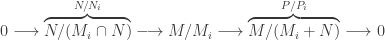
 by the second isomorphism theorem. By
  .
. is surjective, we pick an element of
  . Since
  , the element is represented by a sequence
  in M such that
  . We need to show there is a sequence
  in M such that
 ; we need
  such that
  and
and  . But observe that
  . If we write
  for
for  , then
  works. ♦
 , where
  has the filtration induced from M.
 . From proposition 1 we get an exact sequence
 which is
  for all
  . Thus
  and we are done. ♦
 is a Cauchy sequence, from the
 so as shown in
  . From the above, every Cauchy sequence converges in
  for
for  and
and  . Since
  , we see that m can be represented by an element of M. Thus any non-empty open subset of
  is homeomorphic to the Cantor set:
 .
.
 , so the induced filtration on M/N is also 𝔞-adic. On the other hand, the induced filtration on a submodule N is
  .
. of M is said to be 𝔞-stable if for some n, we have
  for all
  .
. , i.e.
  . Now fix an n such that
 . Taking the inverse limit:
 .
. and
and  ; thus
 . ♦
. ♦

 from multiplication in A. Hence, B(A) has a canonical structure of a
  which gives B(M) a structure of a graded B(A)-module. When A and M are given the 𝔞-adic filtration, we write
  and
and  for their blowup algebra and module.
 for some
  . It follows that
  is a sum of
  where
where  . Hence the map
![A[X_1, \ldots, X_k] \longrightarrow B_{\mathfrak a}(A), \quad X_i \mapsto (x_i \in A_1)](https://s0.wp.com/latex.php?latex=A%5BX_1%2C+%5Cldots%2C+X_k%5D+%5Clongrightarrow+B_%7B%5Cmathfrak+a%7D%28A%29%2C+%5Cquad+X_i+%5Cmapsto+%28x_i+%5Cin+A_1%29&bg=ffffff&fg=333333&s=0&c=20201002)
 Since M is a noetherian A-module, each
  (
( . Now we take the set of
  , as homogeneous elements of B(M) of degree i.
 is an A-linear combination of these generators. Furthermore,
  so
so  generate (over
  is finitely generated over
  ; let
; let  and
and  . We claim that
  for all
  . Since M is filtered, we have
 , regard it as an element of
  and write
  with
with  . Since y and
  are homogeneous, we may assume
  . So
. So  . Write
 , with
  so
so  .
. is a
is a 
 for any
  . A filtered ring is a ring with a designated filtration.
 , in fact each
  is an ideal of A.
 is a
is a  (where
  refers to the grading).
 . E.g. we can take
  and
and  , then
  . More generally, in a
  , we can take
  .
.
 , each
  .
. is said to be filtered if
  for each i.
 is a filtration of M, the induced filtration on N via f is given by
  .
. is a filtration of N, the induced filtration on M via f is given by
  .
. .
.

 and
and  have induced filtrations via quotient module of M and submodule of N. Although
  as A-modules, it is not an isomorphism in the category of filtered A-modules!

 in general.

 such that for each i,
  maps to
  .
. induce an A-linear map
  be its image in
  ; then the map takes
  . From this we see that:
 is injective if and only if
  , in which case we say the filtration is Hausdorff.
 . Although we defined
 in the category of rings. In particular, the canonical map
  is a ring homomorphism.
 , where
 forms a basis for the resulting topology. In fact, d is an
  be a sequence in a filtered module M. We say the sequence is Cauchy if: for any i, there exists n such that
 .
. is Cauchy here if and only if it is Cauchy with respect to the metric of exercise A.3.
 modulo
  . Now define:
 .
. (resp.
  ) are Cauchy sequences in M (resp. in A), then
  and
and  are also Cauchy and we have
 . Given a sequence
  for
for  , let
, let , an element of
  .
. is a Cauchy sequence in A and we write:
 .
. for a prime p. The completion
 is congruent to -1 modulo any
  . Thus
  . In general, an element of
  would have base-2 expansion
  . One easily checks that three times this value is
  , which is -1.
![B = A[X, Y]](https://s0.wp.com/latex.php?latex=B+%3D+A%5BX%2C+Y%5D&bg=ffffff&fg=333333&s=0&c=20201002) and
and  where
where  and check that
  . Note that
 ![\hat B \cong A[[X,Y]]](https://s0.wp.com/latex.php?latex=%5Chat+B+%5Ccong+A%5B%5BX%2CY%5D%5D&bg=ffffff&fg=333333&s=0&c=20201002) , the ring of formal power series with coefficients in A.
, the ring of formal power series with coefficients in A. , where
  and
and  ,
,
![A[[X_1, \ldots, X_n]] := (A[[X_1, \ldots, X_{n-1}]])[[X_n]]].](https://s0.wp.com/latex.php?latex=A%5B%5BX_1%2C+%5Cldots%2C+X_n%5D%5D+%3A%3D+%28A%5B%5BX_1%2C+%5Cldots%2C+X_%7Bn-1%7D%5D%5D%29%5B%5BX_n%5D%5D%5D.&bg=ffffff&fg=333333&s=0&c=20201002)
![\mathbb C[[Y]] \to \hat A](https://s0.wp.com/latex.php?latex=%5Cmathbb+C%5B%5BY%5D%5D+%5Cto+%5Chat+A&bg=ffffff&fg=333333&s=0&c=20201002) is an isomorphism. Geometrically, this means when we project
is an isomorphism. Geometrically, this means when we project  to the Y-axis, the map is locally invertible at the origin.
![A[[X, Y]]](https://s0.wp.com/latex.php?latex=A%5B%5BX%2C+Y%5D%5D&bg=ffffff&fg=333333&s=0&c=20201002) behaves quite differently from
behaves quite differently from ![A[X, Y]](https://s0.wp.com/latex.php?latex=A%5BX%2C+Y%5D&bg=ffffff&fg=333333&s=0&c=20201002) , because as an A-module, it is a countably infinite direct product of copies of A, unlike
, because as an A-module, it is a countably infinite direct product of copies of A, unlike ![B \otimes_A A[[X, Y]] \cong B[[X, Y]]](https://s0.wp.com/latex.php?latex=B+%5Cotimes_A+A%5B%5BX%2C+Y%5D%5D+%5Ccong+B%5B%5BX%2C+Y%5D%5D&bg=ffffff&fg=333333&s=0&c=20201002) for any A-algebra B.
for any A-algebra B.![\mathbb C[[X]] \to \mathbb C[[X, Y]]/(Y^2 - X^3 + X)](https://s0.wp.com/latex.php?latex=%5Cmathbb+C%5B%5BX%5D%5D+%5Cto+%5Cmathbb+C%5B%5BX%2C+Y%5D%5D%2F%28Y%5E2+-+X%5E3+%2B+X%29&bg=ffffff&fg=333333&s=0&c=20201002) is not an isomorphism.
is not an isomorphism.![f(X) \in A[[X]]](https://s0.wp.com/latex.php?latex=f%28X%29+%5Cin+A%5B%5BX%5D%5D&bg=ffffff&fg=333333&s=0&c=20201002) is
is  , then f defines a map
 , we get a ring homomorphism
 ![A[[X]] \to \hat A](https://s0.wp.com/latex.php?latex=A%5B%5BX%5D%5D+%5Cto+%5Chat+A&bg=ffffff&fg=333333&s=0&c=20201002) ,
,  .
. such that

 means every
  for some
  (uniqueness holds up to appending or removal of
  ). Then
  is called the degree-d component of
  .
. ; we write
  . Note that d is unique if
  .
. has A-basis given by the set of monomials
  satisfying
  and
and  .
. is a subring of A and each
  it suffices to show
  ; we may assume
  . Write
  with
with  . Suppose n > 0. For any
  we have
 . Thus
  for any m so we have
  . This gives
  , a contradiction.
 are homogeneous of degrees m and n, then
  is homogeneous of degree m+n. We also have:
 are non-zero elements such that
  and
and  as sums of their components. Let m (resp. m’) be the minimum (resp. maximum) degree for which
  (resp
(resp  ). Similarly, let n (resp. n’) be the minimum (resp. maximum) degree for which
  ). By definition
  . Since ab is homogeneous we have
  and thus
  . So a and b are homogeneous. ♦
 such that ab is homogeneous but a and b are not. [ Hint: come back to this exercise after finishing the whole article. ]
 such that
 .
. with
with  , then
  is called the degree-d component of m.
 ; again write
  .
. , all homogeneous components of n lie in N.
 .
. . Pick a generating set S for N comprising of non-zero homogeneous elements. For each
  with
with  with
with  . Fix
. Fix  and let n’ be the degree-d component of n. Then n’ is the sum of the degree-d components of
  . Hence
 , where
  is the degree-
 component of
  .
. where
where  . Since
  , it is homogeneous of degree i; thus
  is the degree-i component of n and it lies in N.
 to obtain a homogeneous generating set.
 is generated by homogeneous elements, so is
  ; thus
  , if n’ is a homogeneous component of n, then for each i,
  and hence
  . Thus
  is graded. Finally, if S (resp. T) is a generating set of
  is a generating set of
  comprising of homogeneous elements. ♦
 is graded.
 are graded submodules, then
  is a graded ideal.
 .
. . It remains to show M/N is a direct sum of
  .
. with
with  is the sum of images of
  in
in  . So
. So  .
. can be written as
 ![\sum_i [m_i + (N\cap M_i)]](https://s0.wp.com/latex.php?latex=%5Csum_i+%5Bm_i+%2B+%28N%5Ccap+M_i%29%5D&bg=ffffff&fg=333333&s=0&c=20201002) and
and ![\sum_i [m_i' + (N\cap M_i)]](https://s0.wp.com/latex.php?latex=%5Csum_i+%5Bm_i%27+%2B+%28N%5Ccap+M_i%29%5D&bg=ffffff&fg=333333&s=0&c=20201002) . Then
. Then
 so
so  . ♦
. ♦ is a graded ring under the above grading.
 ♦
♦ , so that
 ![A \cong k[X_1, \ldots, X_n]/I(V)](https://s0.wp.com/latex.php?latex=A+%5Ccong+k%5BX_1%2C+%5Cldots%2C+X_n%5D%2FI%28V%29&bg=ffffff&fg=333333&s=0&c=20201002) . If I(V) is homogeneous, then A is a graded ring. In particular, the group of units in A is
. If I(V) is homogeneous, then A is a graded ring. In particular, the group of units in A is  , the multiplicative group
  . This does not work for non-homogeneous I(V), e.g. the unit group of
 ![k[X, Y]/(XY - 1)](https://s0.wp.com/latex.php?latex=k%5BX%2C+Y%5D%2F%28XY+-+1%29&bg=ffffff&fg=333333&s=0&c=20201002) contains
contains  (does equality hold?).
![A = \mathbb C[X, Y, Z]/(Z^2 - X^2 - Y^2)](https://s0.wp.com/latex.php?latex=A+%3D+%5Cmathbb+C%5BX%2C+Y%2C+Z%5D%2F%28Z%5E2+-+X%5E2+-+Y%5E2%29&bg=ffffff&fg=333333&s=0&c=20201002) is not a UFD. Indeed we have the equality
is not a UFD. Indeed we have the equality  in A; we claim that
  are all irreducible. By lemma 2, since Z is homogeneous of degree 1, we can only factor it as a product of a degree-0 and a degree-1 element. But all non-zero degree-0 elements of A are units (see example 1). Similarly
  are irreducible and
  are clearly not associates.
![\mathbb C[W, X, Y, Z]/(Z^2 - W^2 - X^2 - Y^2)](https://s0.wp.com/latex.php?latex=%5Cmathbb+C%5BW%2C+X%2C+Y%2C+Z%5D%2F%28Z%5E2+-+W%5E2+-+X%5E2+-+Y%5E2%29&bg=ffffff&fg=333333&s=0&c=20201002) is not a UFD.
is not a UFD.![\mathbb C[X_1, \ldots, X_n]/(X_1^2 + \ldots + X_n^2)](https://s0.wp.com/latex.php?latex=%5Cmathbb+C%5BX_1%2C+%5Cldots%2C+X_n%5D%2F%28X_1%5E2+%2B+%5Cldots+%2B+X_n%5E2%29&bg=ffffff&fg=333333&s=0&c=20201002) is a UFD for all
is a UFD for all  , as we will see later.
 is a graded submodule of M and
  is a graded submodule of N.
 and
and  with
with  and hence
  is the unique decomposition of f(m) into its homogeneous components. The rest is an easy exercise. ♦
 . Since f is graded, g takes the LHS into
  .
. is also graded. For
  , let
, let  . Write
  is the degree-i homogeneous component of
  we have
  so
so  . ♦
. ♦ be a directed system of rings. Regard them as a directed system of abelian groups (i.e. ℤ-modules) and take the direct limit A.
 , let
, let  be the canonical map.
 , by
, by  and
and  such that
  ,
,  . Now define multiplication in A by
  . This does not depend on our choice of j and
  . Indeed, if we have another index
  such that
  ,
,  , by
, by  greater than i and j such that

 , pick
  such that
  . Then
  .
. , we pick any index
  . ♦
. ♦ in the above proof is well-defined, and
  for all
  for some i. [ Hint:
  is an arbitrary collection of A-algebras. For each finite subset
  , define
  . Define a directed system of
  over the directed set of all finite subsets of I, ordered by inclusion
  . T
. T over
over  , we will write
  for the earlier
  is directed.
 is a multiplicative subset.
 but
but  in general.
 but
but  .
. but
but  in general.
 is a flat B-module.
 .
. if
if  is a diagram of A-modules of type J.
 of B-modules; in particular
  .
. is surjective, then
  is surjective; however, if f is injective
  is not injective in general.
 and
and  . Find an example where the map is not an isomorphism.
 be a projective B-module?
 relations to learn. It turns out most of these constructions can be classified as either “left-adjoint-like” or “right-adjoint-like”, which saves us a whole lot of effort in remembering them.
 .
.
 . [ Take
  and
and  .
. takes a right-exact sequence to a left-exact sequence.
 , the set of all A-linear maps
  , has a natural structure of a B-module.

 is right-adjoint to the forgetful functor
  .
. the coinduced B-module from M.
 is a right-exact functor, but there is a rather huge issue here: the functors are between
  and
and  , the category of diagrams in
  be diagrams of type J. For concreteness, write these diagrams as
 . Let
. Let  be morphisms, written as a collection of
  over
over 

 is concretely described as follows. Take the quotient of
  by all
  , where
  are identified with their images in
  .
. is surjective. Also, composing
  is the zero map so
  . Now write
  for
for  and
and  for
for  .
. represent an element in the kernel of
  . Thus
  is a finite sum of
  . Since
  is surjective, we can write such a term as
 . Since
  is a finite sum of
  , we can replace x by another representative such that
  . Then
  for some
  . ♦
. ♦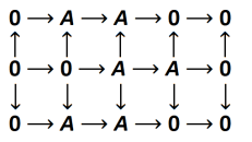
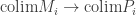
 are identities. The rows are short exact sequences and the squares all commute, but taking the colimit of the columns gives
 , we
, we  whose objects are elements of S, and between any
  ,
,  with equality if and only if
  . Composition is the obvious one.
 , there is a
  such that
  and
and  .
. is called the direct limit and denoted by
 .
.
 if g is a multiple of f. Since S is multiplicative, any {f, g} has an upper bound fg. Hence
  is the direct limit of
  over
over  :
: .
. .
. is a directed system of A-modules over a directed set J. Let
 , with canonical
  for each
  .
. satisfies
  , then there exists
  such that
  .
. for some sufficiently large index j“.
 (with canonical
  ) by relations of the form
 for
for  . But J is a directed set, so we can pick index
  ; then
 , where
  ,
, is a finite sum of the above relations. Pick an index
  is the sum of the images of these relations in
  . But each such relation has image
  in
in  as desired. ♦
 is a directed system of A-modules such that
  are all injective, then
 be directed systems of A-modules and
  be a morphism of the directed systems, i.e. for any
  , we have
  .
. is injective, so is
  .
. and
and  for the canonical maps.
 for
for  . By proposition 2, we have
  for some
 , so
, so  . Since
  is injective we have
  . ♦
. ♦ over J. State and prove an analogue of proposition 2.
 .
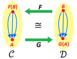
. and
and  are said to be adjoint if we have isomorphisms
 .
.
 and
and  , we have a bijection
 and
and  .
.

 . Similarly for each
  , the contravariant functor
  taking
  is representable.
 take a set S to the free group F(S) on S and
  be the
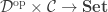
 take a set S to the (commutative) ring
 ![\mathbb \mathbb Z[S] := Z[x_s : s\in S]](https://s0.wp.com/latex.php?latex=%5Cmathbb+%5Cmathbb+Z%5BS%5D+%3A%3D+Z%5Bx_s+%3A+s%5Cin+S%5D&bg=ffffff&fg=333333&s=0&c=20201002) and
and  be the forgetful functor. Again we get
![\mathrm{hom}_{\mathbf{Ring}}(\mathbb Z[S], R) \cong \mathrm{hom}_{\mathbf{Set}}(S, U(R))](https://s0.wp.com/latex.php?latex=%5Cmathrm%7Bhom%7D_%7B%5Cmathbf%7BRing%7D%7D%28%5Cmathbb+Z%5BS%5D%2C+R%29+%5Ccong+%5Cmathrm%7Bhom%7D_%7B%5Cmathbf%7BSet%7D%7D%28S%2C+U%28R%29%29&bg=ffffff&fg=333333&s=0&c=20201002)
 . On the other hand, we have the forgetful functor
  from the canonical ring homomorphism
  . By the universal property of induced B-modules
 . Take functors
  where
where 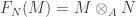 and
and  . In
. In  . This translates to a natural isomorphism
 is left adjoint to
  .
. . Suppose the coproduct of any two objects in
  take
take  and
and  take
take  . By definition of coproduct in categories, we have
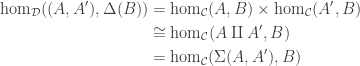
 and
and  . Hence the coproduct functor is left adjoint to the diagonal functor. Dually, the product is right adjoint to the diagonal functor.
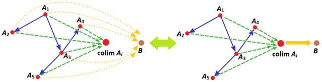
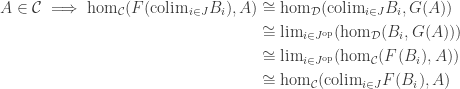
 be this colimit functor. On the other hand, take the diagonal embedding
  which takes an object A to the diagram where all objects are A and all morphisms are
 and object
  .
.
 be the forgetful functor. Find a left adjoint and a right adjoint to U (these are two different functors of course).
 be the inclusion functor, where
  is the category of abelian groups. Find a left adjoint functor to U.
 is left adjoint to
  . If coproducts exist in both categories, then
  because we have natural isomorphisms
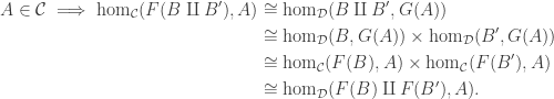
 in
in  .
.
 has no right adjoint.
 has no right adjoint.
 and A-module N, we have

 , for A-module M and B-module N, is an isomorphism of additive groups
 is an exact sequence of A-modules. To prove
  is exact, by

 is a left-exact functor by
  is right-exact.
 , a morphism
  is a natural transformation
  .
. .
.
 is a collection of morphisms
  such that

 which takes a diagram in
  is a diagram of type J. Let
  be the submodule generated by all elements of the form
  over all
  in
in  satisfies our desired universal properties.
 for all
  .
. such that for any
  . The collection of
  induce, by definition of direct sum, a unique map
  such that
  for each
 factors through
  such that
  . Thus for each
  . ♦
. ♦ ,
,  and
and  .
. is a morphism of index categories. Composition then gives:
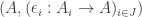
 .
. . If
. If  .
. . Indeed, a morphism between diagrams
  is a natural transformation
  . We let F take this T to
 ,
, by the following tuples
 is of a collection of morphisms
  . Now the new diagrams
  and
and  are the same tuples but with
  and
and  is given by the same collection of
  , except now i runs through
  .
. be a morphism of index categories. Then for any diagram in
  and
and  , we have an induced
 comes with a collection of morphisms
  such that
  for all
  comes with a collection of morphisms
  such that
  for all
  in
in  such that
  for all
  such that
  . ♦
. ♦
 , assuming both objects exist. More generally we have
  .
.

 is an object,
  is a morphism in
  .
.
 , there is a unique morphism
  such that
 .
.
 in a category
 such that
  and, for any pair
  such that
  , there is a unique
  such that
  .
. ).
). . Dually, the same holds for terminal objects. In summary, initial (resp. terminal) objects are unique up to unique isomorphism.
 , whose objects are pairs

 such that
  . Then
  is an (initial / terminal) object in
  which is the coproduct of B and C in the category of A-algebras. But the category of A-algebras corresponds to the
  whose objects are morphisms
  in
in  ,
,  be morphisms in the category
  and
and  is a triplet:
 ,
, is an object,
  ,
,  are morphisms in
  such that for any triplet:
 and morphisms
  satisfying
  , there is a unique morphism
  such that
  and
and  .
.
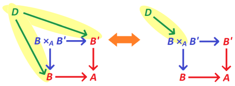
 classifies all morphisms “from” the diagram in red.
 is
is  .
. and
and  in the category
 is the disjoint union of T and T’.
 and
and  be injective group homomorphisms in
  and
and  in the category
  and
and  in the category
  .
. ,
,  be morphisms in
  and
and  in the opposite category
  .
. .
.
 and
and  be functions in
 ,
,  taking
  to
to  respectively.
 and
and  is the inclusion map. Then
 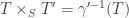 , i.e. the fibre space of
  and
and  are both inclusions. Then
  .
. ,
,  ?
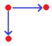
? and the only morphisms are the identities. E.g. the index set {1,2,3} has 3 vertices and one identity arrow for each object.
 be an index category; a diagram of type
  .
. we assign an object
  and to each arrow
  in J, we assign a morphism
  .
.
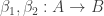
 is not drawn. In particular, identity maps are not drawn. ]
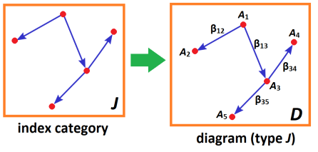
 be a diagram, written as
 .
.
 is an object,
  is a morphism for each
  , we have
  .
.
 , there is a unique morphism
  in
in  .
. .
.
 in a category
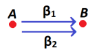
 where
where  is an object such that
  and, for any pair
  satisfying
  , there exists a unique
  such that
 defined as follows. If g = af we take the canonical map
  . Otherwisee there is no map between
  . Prove also that we get a ring isomorphism
  .
. we have
 .
.