[ Warning: this is primarily an expository article, so the proofs are not airtight, but they should be sufficiently convincing. ]
The five platonic solids were well-known among the ancient Greeks (V, E, F denote the number of vertices, edges and faces respectively):
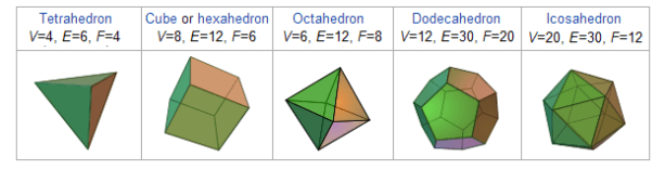
[ Images edited from wikipedia.org. ]
In all cases, we have V–E+F=2. In fact, the same equality holds for any polyhedron which can be “deformed” into the surface of a ball. For example, if we have a pyramid with an n-gon as a base, then V=n+1, E=2n, F=n+1 which gives V–E+F=2. Or, we can glue a pyramid with a square base to a cube (assuming the side lengths match), and obtain V=9, E=16, F=9. Let’s state and prove this result.
Theorem 1. A convex polyhedron whose surface comprises of V vertices, E edges and F faces satisfies V–E+F=2.
Proof
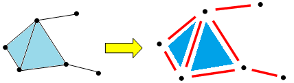
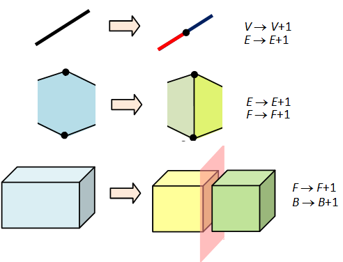
Being convex, the polyhedron can be enclosed in a sphere and its surface projected bijectively to the surface of the sphere. This gives a partition of the sphere’s surface into polygons (called a cellular decomposition). For any two cellular decompositions P and P’, we say that P’ is a refinement of P if all vertices and edges of P are also in P’.
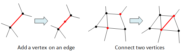
Since any two cellular decompositions have a common refinement, it suffices to show that if P’ is a refinement of P, then they have the same V–E+F. Now any refinement may be obtained from a sequence of steps, each of which is one of the two following types:

The left step changes (V, E, F) to (V+1, E+1, F) since it adds a vertex and an edge without introducing any new face. The right step changes (V, E, F) to (V, E+1, F+1). In both cases, there is no change to V–E+F. Hence this value is constant across all decompositions of the sphere and picking any single example gives V–E+F=2. ♦

The above proof, while simple, has a few hidden pitfalls for the unwary. For more details, the interested reader may refer to Imre Lakatos’ book “Proofs and Refutations” for a rather in-depth look at the underlying issues as well as their historical relevance.
The simple V–E+F formula has some interesting applications.
Example 1
Let’s prove that there are at most 5 platonic solids. Suppose we have a polyhedron with F faces, each of which is an n-gon with m edges meeting at each vertex. Then E = Fn/2 and V = 2E/m. The formula V–E+F = 2 gives

Since m, n ≥ 3, it’s easy to see that this inequality only holds for (m, n) = (3, 3), (3, 4), (3, 5), (4, 3), (5, 3), after which one can show that each case has at most one platonic solid.
Example 2
The utility graph cannot be drawn on the sphere (and hence on the plane) without intersecting edges. Indeed, if it could, we would have V=6, E=9, and so F = 2-V+E = 5. But since the graph has no triangles, each face has at least 4 edges and this gives at least 5×4/2 = 10 edges, which is a contradiction.
Exercise. Prove that the complete graph with 5 vertices cannot be drawn on the sphere without intersecting edges. Read up on planar graphs.

Other Surfaces
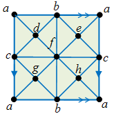
A closer look at the proof of thereom 1 indicates that V–E+F is constant for any cellular decomposition of a suitably nice surface. For example, on the surface of a torus (doughnut), the following decomposition gives – after unfolding – four faces of rectangles.
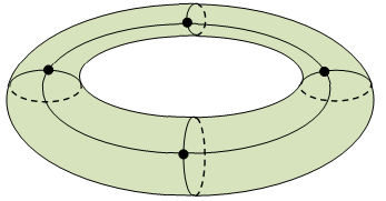
Hence V=4, E=8, F=4, and V–E+F=0. This suggests that V–E+F is an indication of the global topological property of the shape. We will call this the Euler characteristic of the surface. If we partition the surface of a two-holed doughnut, we find that its Euler characteristic is -2, and so on. This suggests the following.
Proposition 2.
The Euler characteristic of the surface of a g-holed torus is 2-2g.

We will leave the proof to the reader since it is a matter of straightforward computation.
In fact, we don’t have to restrict ourselves to smooth surfaces (the formal terminology is called closed manifolds); let’s look at some surfaces with edges.
Example 3
For a square, we have V=4, E=4, F=1, so the Euler characteristic = 1. Or, we can partition it into two triangles and get V=4, E=5, F=2.
Example 4
Consider the Möbius strip which is obtained by gluing a pair of opposite sides of a square by flipping over one edge. By dividing the square into two triangles, we get V=2 (since A=D, B=C), E=4 (since AC=DB) and F=2, so the Euler characteristic is 0.

Example 5
The Klein bottle is obtained by gluing the two opposite sides of the Möbius strip together, i.e. AB to CD (preserving the direction). This gives V=1 (since A=B=C=D), E=3 and F=2 so the Euler characteristic is 0.
Example 6
The projective plane is obtained by gluing the oppposite edges of a square in opposite directions, as follows.

This gives V=2 (since the opposite vertices of the square are glued together), E=2, F=1, and the Euler characteristic is 1.
Example 7
In fact, you don’t even need the surface to be connected. Indeed, it’s clear that if X is the topological disjoint union of M and N, and χ(X) denotes the Euler characteristic of X, then

More generally, we have the following result:
Principle of Inclusion and Exclusion. Suppose X is the union of M and N. Then  .
.
Proof
Find a cellular decomposition of M and of N, then form a decomposition of X which is a refinement of both. The result then follows easily by counting the number of times each vertex/edge/face appears in M and N. ♦
Exercise
- Draw the utility graph on the surface T of a torus such that the edges do not intersect. [Solution.]
- Do the same with the complete graph on 5 vertices.
- Find the largest n for which we can embed the complete graph on n vertices on T.
- Read up on toroidal graphs, or more generally, topological graph theory.
Other Dimensions
The Euler characteristic can be generalised to objects of arbitrary dimensions. For one dimensional objects, they can be represented by graphs. E.g. the nuclear disarmament symbol can be represented by a graph with V=5 vertices and E=8 edges so the Euler characteristic is now χ = V–E = -3.

Graphically, χ = 1-c where c is the number of “holes” in the diagram. It’s easy to show that the Euler characteristic χ = V–E for 1-dimensional objects is well-defined, i.e. independent of the graph representation we pick. Indeed, the proof is identical to before (that of theorem 1), except that in this case we can only add a vertex to an edge, since connecting two vertices completely changes the object.
Thus, for a general geometric object, we can add a vertex to break an edge into two, or an edge to break a face into two, or a face to divide a block into two, … , as illustrated by the following (B denotes the number of 3-dimensional blocks):

This shows that for a 3-dimensional object, its Euler characteristic χ = V–E+F–B is constant. Clearly we can generalise this to arbitrarily many dimensions: if a cellular decomposition of M comprises of  cells of dimension i, then its Euler characteristic

is independent of the decomposition.
Example 8
Consider a solid cube. We already know that the surface of a cube satisfies V–E+F=2. Hence, the solid cube has χ = 2-1 = 1.
Example 9
Now consider a solid cube with a small cubical hole at the centre. We could partition this solid as a union of 6 pieces of the form:
which gives us B=6, F=24, E=32, V=16 (after some careful counting!) and so χ=2.
Or, we could also use the principle of inclusion and exclusion (whose proof clearly generalises to any geometric shapes). If M is the above cube with a hole, and N is the small cube at the centre, then their union is the large cube and their intersection is the surface of a cube, so we have:

which we already know is 2.
Example 10
Consider the case of dimension 0, where we have a discrete set of points. The Euler characteristic is then the cardinality of this set (i.e. number of elements in it).
Simplicial Complexes
Let us now define in a more precise manner what objects we’re looking at. Heuristically, we start with a set S of points. A simplicial complex is then represented by a collection C of subsets of S such that if  , then every subset of T also lies in C.
For example, if S = {1, 2, 3, 4} and C = { Ø, {1}, {2}, {3}, {4} {1,2}, {2,3}, {1,3}, {2,4}, {1,2,3} }, then the corresponding simplicial complex is:

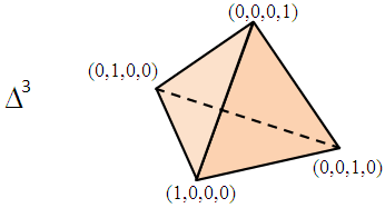
The formal topological definition is as follows: the n-dimensional simplex is the set

or its affine transform. For example, here’s a 3-dimensional simplex.
The boundary of  comprises of (n+1) simplices of dimension (n-1), each corresponding to an 0 ≤ i ≤ n, for which we take the set of
  satisfying
  Now take each element
  and form the corresponding simplex

Now the simplicial complex for Σ is the topological space which is the subspace  In other words, the objects we’re looking are topological spaces which are homeomorphic to a simplicial complex. Note that even though the construction of a simplicial complex only uses line segments, triangles, tetrahedrons, and their higher-dimensional counterparts, its cellular decomposition may use more general shapes such as quadrilaterals, pentagons, cubes etc.
Note: simplicial complexes are somewhat restrictive. A more general theory involves CW-complexes. The differences are subtle, and while CW-complexes may define some structures which are not homeomorphic to any simplicial complex (see here for some anomalous examples), the two theories are equivalent at the level of homotopic equivalence, which we will define in the next article.
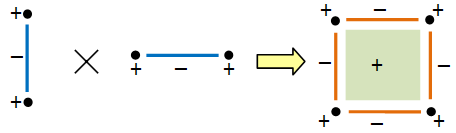
Multiplicativity of χ
Finally, we have the following result.
Theorem. If M and N are geometric objects, we have χ(M × N) = χ(M) × χ(N).
Proof
First, note that each cellular decomposition of a geometric object gives a disjoint union of the underlying set of points:
Write  and
and  as disjoint unions in this way (some of the Mi‘s or Nj‘s may have the same dimension). Then their Euler characteristics are given by:

Now  and
and  so the Euler characteristic of M × N is:

which is χ(M)χ(N). ♦
Here’s a graphical representation of the above proof.

![K[G] \cong \prod_{i=1}^k M_{n_i}(K)](https://s0.wp.com/latex.php?latex=K%5BG%5D+%5Ccong+%5Cprod_%7Bi%3D1%7D%5Ek+M_%7Bn_i%7D%28K%29&bg=ffffff&fg=333333&s=0&c=20201002)
![|G| = \dim_K K[G] = \sum_{i=1}^k \dim(V_i)^2](https://s0.wp.com/latex.php?latex=%7CG%7C+%3D+%5Cdim_K+K%5BG%5D+%3D+%5Csum_%7Bi%3D1%7D%5Ek+%5Cdim%28V_i%29%5E2&bg=ffffff&fg=333333&s=0&c=20201002)

, where V runs through all simple K[G]-modules, forms an orthonormal basis of the space of class functions.

![\alpha = \sum_{g\in G} f(g^{-1})\cdot g \in K[G].](https://s0.wp.com/latex.php?latex=%5Calpha+%3D+%5Csum_%7Bg%5Cin+G%7D+f%28g%5E%7B-1%7D%29%5Ccdot+g+%5Cin+K%5BG%5D.&bg=ffffff&fg=333333&s=0&c=20201002)
![\alpha g = g\alpha \in K[G]](https://s0.wp.com/latex.php?latex=%5Calpha+g+%3D+g%5Calpha+%5Cin+K%5BG%5D&bg=ffffff&fg=333333&s=0&c=20201002)


![\mathbf{R}[G] \cong V_{\text{triv}} \oplus V_i \oplus V_j \oplus V_k \oplus W](https://s0.wp.com/latex.php?latex=%5Cmathbf%7BR%7D%5BG%5D+%5Ccong+V_%7B%5Ctext%7Btriv%7D%7D+%5Coplus+V_i+%5Coplus+V_j+%5Coplus+V_k+%5Coplus+W&bg=ffffff&fg=333333&s=0&c=20201002)
![\tau = \chi_{\mathbf{R}[G]} - \chi_{\text{triv}} - \chi_i - \chi_j - \chi_k = 2\chi.](https://s0.wp.com/latex.php?latex=%5Ctau+%3D+%5Cchi_%7B%5Cmathbf%7BR%7D%5BG%5D%7D+-+%5Cchi_%7B%5Ctext%7Btriv%7D%7D+-+%5Cchi_i+-+%5Cchi_j+-+%5Cchi_k+%3D+2%5Cchi.&bg=ffffff&fg=333333&s=0&c=20201002)


so
and so ρ(g) has eigenvalues ±√-1. From the character table, its trace is zero so the eigenvalues are +√-1 and -√-1.


![\mathbf{R}[G] \cong \mathbf{R} \times \mathbf{R} \times \mathbf{R} \times\mathbf{R} \times D](https://s0.wp.com/latex.php?latex=%5Cmathbf%7BR%7D%5BG%5D+%5Ccong+%5Cmathbf%7BR%7D+%5Ctimes+%5Cmathbf%7BR%7D+%5Ctimes+%5Cmathbf%7BR%7D+%5Ctimes%5Cmathbf%7BR%7D+%5Ctimes+D&bg=ffffff&fg=333333&s=0&c=20201002)

 taking
  is K-bilinear, so it induces a linear map
  taking

 It is given the structure of a K[G]-module as follows:
 be the space of K-linear maps V → W. It is given the structure of a K[G]-module as follows:
 when V and W are finite-dimensional. The LHS has a K[G]-module structure via (iv) while the RHS has a K[G]-module structure via (ii) and (iii). It is easy to check that they are consistent. ]

 since
since  for any square matrices A and B with B invertible. Generally, a function χ : G → K is said to be a class function if
  for any g, h in G. Thus characters are class functions.

 be the space of G-invariant vectors. Then:
 . We have:
 which proves our lemma. ♦
 The lemma says that the dimension of the space UG is:
 ; thus f is G-invariant if and only if
  for all g in G, v in V. In short, the space of G-invariant elements of U is precisely the space of intertwining operators V→W, or equivalently, K[G]-module homomorphisms V→W.
 , where “g” here is an abstract symbol for each element g of G. Thus, K[G] has dimension |G| over K. Now K[G] has a ring structure obtained from group multiplication, where the algebra product σ⋅τ is precisely the group product, i.e. an element of G. For example, multiplication in Q[S3] gives
 , of G to the group of invertible K-linear maps M→M; such a ρ is called a representation of G over K. Indeed, if M is a K[G]-module, then considering how elements g ∈ K[G] acts on M (for g ∈ G), we obtain a homomorphism
 , then this gives M the structure of a K[G]-module by letting
  (
( ) take m ∈ M to

 is given by:
 be the homomorphism taking
  to the linear map
 for any
  Now M is a module over R[S3], where, e.g. a(1, 2) + b(1, 3, 2) takes the point (x, y, z) to (ay+by, ax+bz, az+bx) so its corresponding matrix is
  assuming elements of M are written as column vectors.
![q : K[G] \to K[G], \quad q(\alpha) := \frac 1 {|G|} \sum_{g\in G} g\cdot p(g^{-1} \alpha)](https://s0.wp.com/latex.php?latex=q+%3A+K%5BG%5D+%5Cto+K%5BG%5D%2C+%5Cquad+q%28%5Calpha%29+%3A%3D+%5Cfrac+1+%7B%7CG%7C%7D+%5Csum_%7Bg%5Cin+G%7D+g%5Ccdot+p%28g%5E%7B-1%7D+%5Calpha%29&bg=ffffff&fg=333333&s=0&c=20201002) for
for ![\alpha \in K[G].](https://s0.wp.com/latex.php?latex=%5Calpha+%5Cin+K%5BG%5D.&bg=ffffff&fg=333333&s=0&c=20201002)
 and since p(α) = α for all α in I, the result follows. Together with property 1, this means im(q) = I.
![K[G] \cong \prod_{i=1}^k M_{n_i}(D_i)](https://s0.wp.com/latex.php?latex=K%5BG%5D+%5Ccong+%5Cprod_%7Bi%3D1%7D%5Ek+M_%7Bn_i%7D%28D_i%29&bg=ffffff&fg=333333&s=0&c=20201002) and letting
and letting ![m_i = [D_i : K]](https://s0.wp.com/latex.php?latex=m_i+%3D+%5BD_i+%3A+K%5D&bg=ffffff&fg=333333&s=0&c=20201002) gives us
gives us![|G| = \dim_K K[G] = \sum_{i=1}^k n_i^2 m_i](https://s0.wp.com/latex.php?latex=%7CG%7C+%3D+%5Cdim_K+K%5BG%5D+%3D+%5Csum_%7Bi%3D1%7D%5Ek+n_i%5E2+m_i&bg=ffffff&fg=333333&s=0&c=20201002) ,
,
 is a division ring and
  is the ring of n × n matrices with entries in D. Furthermore, the list of
  is unique up to permutation, and isomorphism class of

 are pairwise non-isomorphic.
  is zero if M and M’ are not isomorphic, and is a division ring otherwise.
 and
and  by the universal properties of direct sum and product. When we have finitely many terms, the direct sum is the direct product. ]
 , where
 ]
]
 is either 0 (if i ≠ j) or isomorphic to
  , where
  is a division ring. In conclusion:
 for division rings
  corresponds to composition of endomorphisms
  . ]
. ] , for division ring D, has a unique simple module up to isomorphism, namely
  .
.
 , there are exactly k simple modules up to isomorphism, each simple module occurs
  . This shows that we can recover
  is. Another of saying this is: R is “left semisimple” iff it is “right semisimple”.
 a submodule. Then we can find simple submodules
  (indexed by
  ) such that
 where
where  and only finitely many terms are non-zero.
 ). [ For those who worry about set-theoretic validity, note that the collection of all such ∑ forms a bona fide set. ]
 is a chain: i.e. for any
  either
  or
or  Let
Let  let us show that
  is a direct sum.
 for some
  But this is a finite sum, so the equality already holds in some
  (since the
  , pick
  Since M is a sum of simple submodules, write
 , where each Mk is simple.
 we have
  for some k. But this means
  is a proper submodule of Mk, and must be zero (since Mk is simple). Hence
  is a direct sum, so we could have added the simple module Mk to the collection ∑, contradicting its maximality. Thus,
  and we’re done. ♦
 is a semisimple submodule of a module M, then so is
 is a sum of simple modules; by definition so is N. ♦
 .
. . ♦
. ♦ is a direct sum of simple modules. ♦
 as a direct sum of simple left ideals. Then any simple module M is isomorphic to some
  for a single simple module N; this just means N is the only simple R-module up to isomorphism. ]
 are both simple,
  or an isomorphism. If all
  , then so is
  which is absurd. Hence some
  is an isomorphism, which proves the first statement.
 only finitely many of the modules are non-zero.
  where
where 
 gives:
 . ♦
. ♦ . Is this semisimple? [ Answer:
  , we often cannot find a
  such that
  and N + P = M, which just means that every element of M is uniquely writable as x+y, with x in N and y in P). A good example is given by N = 2Z, M = Z; for any other submodule P of Z, we either get P=0 or a non-zero module which must necessarily intersect N.
 and
and  we have the multiplication
  . This ensures that multiplication-by-r followed by multiplication-by-s is simply multiplication-by-sr, since s(rm) = (sr)m. In the case of right modules, this would have been multiplication-by-rs. ]
 , we have
  ]
] , we must have P = N or P = M. From the correspondence between (a) submodules of M/N and (b) submodules of M containing N, we conclude that N is maximal iff M/N is simple. ]
 Its image is a non-zero submodule of M so must be the whole of M. Thus f is surjective and
  ♦
♦ is a homomorphism of simple modules, then either f=0 or f is an isomorphism. In particular, the ring
  is a division ring for a simple module M.
 and
and  ? [ Answer:
  Let M be the space R2 and R acts on M via multiplying matrix with vector. Find a simple submodule of M. [ Answer:

 , then the boundary map is additive:
  as can be seen in the following diagram:
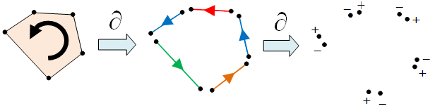
 where
where  are i-dimensional cells and
  These sums are formal in the sense that we merely treat them symbolically; the set of such sums forms a real vector space
  via the following operations
 ;
; .
.
 is the zero map. It follows from basic linear algebra that we have
  as subspaces of
 .
.

 is isomorphic to
  for j = i+1, i, i-1, i-2.
 is spanned by a single element
 is spanned by
  is the full space spanned by {
 and
and  is spanned by

 instead of vector spaces
  , where M is the underlying object and i=0, 1, 2, … .
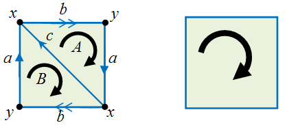

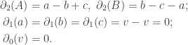
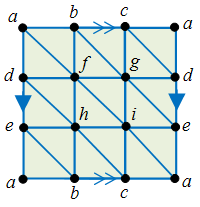
 so the second homology group is
  Next,
Next,  has Z-basis a+b+c and a–c+b, or equivalently, a+b+c and 2c. On the other hand,
  has Z-basis a+b and c. Thus, the resulting group quotient is
  Finally,
  has basis x–y while
  has basis x, y, so the homology group is
 and
and  Thus, the homology groups may differ even if the Betti numbers are the same, but computing the homology groups is a little harder than finding the Betti numbers. This form of homology is known as cellular homology.
![\Delta = [ v_0, v_1, \ldots, v_m ]](https://s0.wp.com/latex.php?latex=%5CDelta+%3D+%5B+v_0%2C+v_1%2C+%5Cldots%2C+v_m+%5D&bg=ffffff&fg=333333&s=0&c=20201002) with its boundary given by:
with its boundary given by:![\partial_i([v_0, v_1, \ldots, v_m]) := \sum_{i=0}^m (-1)^i [v_0, \ldots, \hat{v_i}, \ldots, v_m],](https://s0.wp.com/latex.php?latex=%5Cpartial_i%28%5Bv_0%2C+v_1%2C+%5Cldots%2C+v_m%5D%29+%3A%3D+%5Csum_%7Bi%3D0%7D%5Em+%28-1%29%5Ei+%5Bv_0%2C+%5Cldots%2C+%5Chat%7Bv_i%7D%2C+%5Cldots%2C+v_m%5D%2C&bg=ffffff&fg=333333&s=0&c=20201002)
 . E.g.
 ![\partial_2([a, b, c]) = [b,c] - [a,c] + [a,b].](https://s0.wp.com/latex.php?latex=%5Cpartial_2%28%5Ba%2C+b%2C+c%5D%29+%3D+%5Bb%2Cc%5D+-+%5Ba%2Cc%5D+%2B+%5Ba%2Cb%5D.&bg=ffffff&fg=333333&s=0&c=20201002) As an exercise, check that under this definition, we have
As an exercise, check that under this definition, we have 
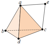
![\partial_2([a, c, d]) = [c,d] - [a,d] + [a,c],](https://s0.wp.com/latex.php?latex=%5Cpartial_2%28%5Ba%2C+c%2C+d%5D%29+%3D+%5Bc%2Cd%5D+-+%5Ba%2Cd%5D+%2B+%5Ba%2Cc%5D%2C&bg=ffffff&fg=333333&s=0&c=20201002)
![\partial_1([a,e]) = [e] - [a]](https://s0.wp.com/latex.php?latex=%5Cpartial_1%28%5Ba%2Ce%5D%29+%3D+%5Be%5D+-+%5Ba%5D&bg=ffffff&fg=333333&s=0&c=20201002) and
and ![\partial_0([d]) = 0.](https://s0.wp.com/latex.php?latex=%5Cpartial_0%28%5Bd%5D%29+%3D+0.&bg=ffffff&fg=333333&s=0&c=20201002) Now it suffices to obtain the homology groups from the sequence
Now it suffices to obtain the homology groups from the sequence  which is left as an exercise for the reader.

 , we get
![\begin{aligned}\sum_i (-1)^i b_i(M) &= \sum_i (-1)^i\dim(\text{ker}(\partial_i)) - (-1)^i\sum_i\dim(\text{im}(\partial_{i+1}))\\ &=\sum_i (-1)^i \dim(\text{ker} (\partial_i)) + \sum_i (-1)^{i+1}\dim( \text{im}(\partial_{i+1})) \\ &=\sum_i (-1)^i [\dim(\text{ker} (\partial_i)) + \dim(\text{im}(\partial_i))] \\ &= \sum_i (-1)^i |S_i| =\chi(M)\end{aligned}](https://s0.wp.com/latex.php?latex=%5Cbegin%7Baligned%7D%5Csum_i+%28-1%29%5Ei+b_i%28M%29+%26%3D+%5Csum_i+%28-1%29%5Ei%5Cdim%28%5Ctext%7Bker%7D%28%5Cpartial_i%29%29+-+%28-1%29%5Ei%5Csum_i%5Cdim%28%5Ctext%7Bim%7D%28%5Cpartial_%7Bi%2B1%7D%29%29%5C%5C+%26%3D%5Csum_i+%28-1%29%5Ei+%5Cdim%28%5Ctext%7Bker%7D+%28%5Cpartial_i%29%29+%2B+%5Csum_i+%28-1%29%5E%7Bi%2B1%7D%5Cdim%28+%5Ctext%7Bim%7D%28%5Cpartial_%7Bi%2B1%7D%29%29+%5C%5C+%26%3D%5Csum_i+%28-1%29%5Ei+%5B%5Cdim%28%5Ctext%7Bker%7D+%28%5Cpartial_i%29%29+%2B+%5Cdim%28%5Ctext%7Bim%7D%28%5Cpartial_i%29%29%5D+%5C%5C+%26%3D+%5Csum_i+%28-1%29%5Ei+%7CS_i%7C+%3D%5Cchi%28M%29%5Cend%7Baligned%7D&bg=ffffff&fg=333333&s=0&c=20201002)
 . Recall that the principle of inclusion and exclusion allows us to compute the Euler characteristics of X from those of M, N and M ∩ N. The question is: what about Betti numbers and homology groups? We would very much like to say
  but we would be lying if we did. Instead, we have the extended exact sequence:
 we have
  Also, the direct sum
  of two groups is simply their product. ]
 then maps chains of M to those of
  Clearly, if an m-chain D of M satisfies ∂D = 0, so does its image in
  is of the form ∂E’, where E’ is the image of E in
  induces a map of homology groups:
 and similarly
 and
and  are injective, in general
  and
and  are not. ] Likewise, the inclusions
  and
and  induce
  and
and  Now we define:
 as the map
 ![[D] \mapsto ({j_M}_*([D]), -{j_N}_*([D]))](https://s0.wp.com/latex.php?latex=%5BD%5D+%5Cmapsto+%28%7Bj_M%7D_%2A%28%5BD%5D%29%2C+-%7Bj_N%7D_%2A%28%5BD%5D%29%29&bg=ffffff&fg=333333&s=0&c=20201002) ,
, as the map
 ![[D] \mapsto {i_M}_*([D]) + {i_N}_*([D]).](https://s0.wp.com/latex.php?latex=%5BD%5D+%5Cmapsto+%7Bi_M%7D_%2A%28%5BD%5D%29+%2B+%7Bi_N%7D_%2A%28%5BD%5D%29.&bg=ffffff&fg=333333&s=0&c=20201002)

 This is the union of
 and
and 
 The long exact sequence above thus gives (together with
  since we’re dealing with two or three-dimensional objects here):
 and hence the full 3-simplex on [0, 1, 2, 3], it is easy to check that they have trivial homology in dimensions ≥ 1. On the other hand, M ∩ N is homeomorphic to the surface of a cube so we get:
 since it’s easy to check that
  is injective.


 is a basis of the quotient space V/W, then the vi‘s, together with a basis
  of W, form a basis of V:
 for some
  , its image in V/W gives
 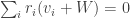 and thus each
  is zero. This gives
  ; since
  This proves that
  is linearly independent.
 . Its image v+W in V/W can be written as a linear combination
  for some
  Hence
Hence  and can be written as a linear combination of
  So v can be written as a linear combination of
 and let f : V → W take the tuple
  Then f is injective but not surjective.
 , in which case we can identify
  via
via  Let’s restrict ourselves to the case of finite free modules, i.e. modules with finite bases. If
  and
and  the group of homomorphisms is identified with
  in terms of b × a matrices in R.
 of M and
  of N. We have:
 and
and 
 and
and  where x is an indeterminate here. The map f : M → N given by f(p(x)) = dp/dx is easily checked to be R-linear.
 Hence, the matrix corresponding to these bases is
 ;
; ;
;

 ;
;
 Replacing the basis by {-1, 1+√2} would give us:
 as an R-module isomorphism. What about Hom(M, R) then?
 This is a
  , then the resulting
  takes
takes  .
.
 takes m to
  which is the image of
  acting on m.
 is called the dual because it’s a right module instead of a left one. Note that if N were a right-module, the resulting space Hom(N, R) of all right-module homomorphisms would give us a left module
  It’s not true in general that
  but it holds for finite-dimensional vector spaces over a division ring.
 which takes (f, v) to f(v). Fixing f, we get a map
  which is a left-module homomorphism. Fixing v, we get a right-module homomorphism
  since (f·r) corresponds to the map
  by definition. This gives a left-module homomorphism
 . But if
  , we can extend {v} to a basis of V. Define a linear map f : V → D which takes v to 1 and all other basis elements to 0. Then
  so
so  This shows that
  is injective and thus an isomorphism. ♦
 What’s wrong with this definition? [ Answer:
  is a basis of V. Let
  (i = 1, …, n) be linear maps defined as follows:
 This is called the dual basis for
 is linearly independent. For that, we write
  for some
  (recall that V* is a
 and
and  we can write
  and
and  for some
  Then
Then
 , there’s a natural inner product given by the usual dot product which is inherent in the geometry of the space. However, for generic vector spaces, it’s hard to find a natural inner product. E.g. what would one be for the space of all polynomials of degree at most 2? Thus, the dual space provides a “cheap” and natural way to get an inner product.
 over the reals R=R. Examples of elements of V* are:
 which takes
  ;
; which takes
  ;
; which takes
  .
. be a basis of V and
  be its dual basis for V*. Denote the dual basis of
  in V**. Prove that under the isomorphism
  , we have
 be a basis of V and
  is denoted M.
 be the dual basis of
  be the dual basis of
  is the transpose of M.
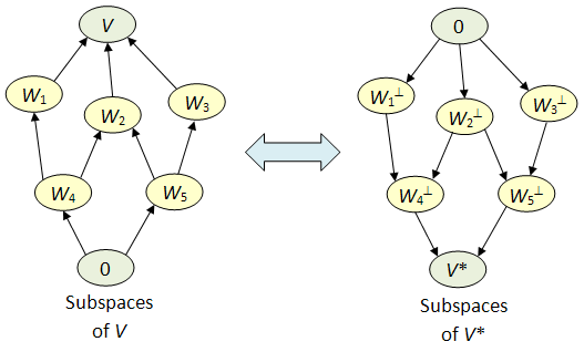
 is a subspace, define
 is a subspace, define
 is a subspace of V*;
 is a subspace of V;
 , then
  ;
; , then
  ;
; and
and  .
. is the subspace of V generated by W.
 . Likewise if
 of W and extend it to a basis
  be the dual basis.
 write
write  where each
  Since v is outside W,
  for some j>k. This gives
  and
and  since j>k. Hence
  and we have
 . ♦
. ♦
 ;
; naturally.
 This proves our claim. ♦