From Euler Characteristics to Cohomology (II)

Boundary Maps

Here’s a brief recap of the previous article: we learnt that in refining a cell decomposition of an object M, we can, at each step, pick an i-dimensional cell and divide it in two. In this way, we introduce an additional i-dimensional cell and an (i-1)-dimensional cell.

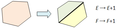
Hence even after successive steps, the Euler characteristic $\chi(M) := \sum_i (-1)^i n_i$ , where n_i denotes the number of i-dimensional cells, is constant. So χ(M) is independent of the cell decomposition we pick for M and can be used to distinguish between topological spaces, i.e. if χ(M)≠χ(N) then M and N are not homeomorphic as topological spaces.

In fact, it is possible to obtain even finer distinguishing characteristics for the topology of M, known as Betti numbers. For starters, consider the boundary function ∂ which takes a cell to its boundary ∂C, while taking into account its orientation. If C is i-dimensional, then ∂C is a union of (i-1)-dimensional cells. For example, in the following diagram, ∂C can be expressed as a sum of 5 edges:

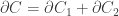
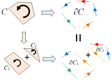
The critical observation is that when we partition a cell into two, written as $C \mapsto C_1 + C_2$ , then the boundary map is additive: $\partial C = \partial C_1 + \partial C_2$ as can be seen in the following diagram:

since the two edges which are equal but in opposite directions cancel each other out. The next property we note is that ∂(∂C) = 0, as illustrated by the following diagram.

Betti Numbers

This suggests the following: let S_i denote the set of i-dimensional cells in the decomposition. An i–chain is defined as a formal sum $D = \alpha_1 T_1 + \alpha_2 T_2 + \dots + \alpha_k T_k,$ where $T_1, \ldots, T_k\in S_i$ are i-dimensional cells and $\alpha_1, \ldots, \alpha_k\in \mathbb{R}.$ These sums are formal in the sense that we merely treat them symbolically; the set of such sums forms a real vector space $\mathbb{R}^{S_i}$ via the following operations

addition: $\left(\sum_i \alpha_i T_i\right) +\left(\sum_i \beta_i T_i\right) = \sum_i (\alpha_i + \beta_i) T_i$ ;
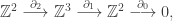
scalar multiplication: $c\cdot \left(\sum_i \alpha_i T_i\right) = \sum_i (c\alpha_i) T_i$ .

The boundary map then gives a linear map:

$\partial_i : \mathbb{R}^{S_i} \to \mathbb{R}^{S_{i-1}},$

such that the composition $\partial_{i}\circ\partial_{i+1} : \mathbb{R}^{S_{i+1}} \to \mathbb{R}^{S_{i-1}}$ is the zero map. It follows from basic linear algebra that we have $\text{im}(\partial_{i+1}) \subseteq \text{ker}(\partial_i)$ as subspaces of $\mathbb{R}^{S_i}.$

Definition. The i-th Betti number, denoted b_i, is the dimension of the quotient $\text{ker}(\partial_i)/\text{im}(\partial_{i+1})$ .

We’ll briefly justify why this definition is independent of our choice of cell decomposition. It suffices to reduce to the case where we partition an i-dimensional cell $C \mapsto C_1 + C_2$ and thus add an (i-1)-dimensional cell D.

The boundary maps are then modified by adding the following relations:

$\begin{aligned} \partial'_{i+1} &= s\circ\partial_{i+1},\ \mbox{ where } s(C) = C_1 + C_2\\ \partial_i'(C_1) &= S + D, \ \partial_i'(C_2) = T - D, \ \mbox{ where } S+T = \partial_i(C)\\ \partial_{i-1}'(D) &= \ldots\end{aligned}$

from which we can show that $\text{ker}(\partial'_j)/\text{im}(\partial'_{j+1})$ is isomorphic to $\text{ker}(\partial_j)/\text{im}(\partial_{j+1})$ for j = i+1, i, i-1, i-2.

Sample Computation: Torus

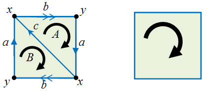
Consider the torus, which is obtained by gluing the opposite sides of a square together in the same direction:

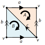
The above cellular decomposition then comprises of the following cells:

2-cells : {A, B}, oriented in clockwise;
1-cells : {a, b, c}, with orientation as above;
0-cells : {v}, since all four vertices of the square are glued together.

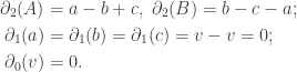
Then we have the following relations:

$\begin{aligned} \partial_2(A) &= a - b + c,\ \partial_2(B) = b - c - a; \\ \partial_1(a) &= \partial_1(b) = \partial_1(c) = v - v = 0;\\ \partial_0(v)&= 0.\end{aligned}$

Now we can easily compute the Betti numbers of the torus.

First, $\text{ker}(\partial_2)$ is spanned by a single element A+B so it has dimension 1. Thus $b_2 = 1-0 = 1.$
Next, $\text{im}(\partial_2)$ is spanned by a+c–b and has dimension 1. And $\text{ker}(\partial_1)$ is the full space spanned by {a, b, c}, so $b_1 = 3-1 = 2.$
Finally, $\text{im}(\partial_1) =0$ and $\text{ker}(\partial_0)$ is spanned by v and has dimension 1, so $b_0 = 1-0 = 1.$

Exercise

Verify the Betti numbers of the following surfaces:

Homology Groups

In fact, by considering the abelian groups $\mathbb{Z}^{S_i}$ instead of vector spaces $\mathbb{R}^{S_i}$ and taking group quotients instead of vector space quotients, one can obtain an even finer distinguisher of topological spaces. The resulting groups are called homology groups and denoted by $H_i(M)$ , where M is the underlying object and i=0, 1, 2, … .

For example, consider the projective plane and the square which have the same Betti numbers.

If we let M be the projective plane on the left, we get:

$\mathbb{Z}^2 \stackrel{\partial_2}\longrightarrow\mathbb{Z}^3 \stackrel{\partial_1}\longrightarrow\mathbb{Z}^2 \stackrel{\partial_0}\longrightarrow 0,$

$\partial_2:\begin{matrix}A\mapsto a+b+c,\\B\mapsto a-c+b\end{matrix}, \qquad \partial_1: \begin{matrix} a\mapsto x-y,\\ b\mapsto y-x, \\ c\mapsto x-x=0\end{matrix}, \qquad \partial_0: \begin{matrix} x\mapsto 0, \\ y\mapsto 0.\end{matrix}$

We still have $\text{ker} \partial_2 = 0$ so the second homology group is $H_2(M) = 0.$ Next, $\text{im} \partial_2$ has Z-basis a+b+c and a–c+b, or equivalently, a+b+c and 2c. On the other hand, $\text{ker}\partial_1$ has Z-basis a+b and c. Thus, the resulting group quotient is $H_1(M) = \mathbb{Z}/2.$ Finally, $\text{im}\partial_1$ has basis x–y while $\text{ker} \partial_0$ has basis x, y, so the homology group is $H_0(M) = \mathbb{Z}.$

On the other hand, we leave it to the reader to check that if N is the square, then $H_2(N) = H_1(N) = 0$ and $H_0(N) = \mathbb{Z}.$ Thus, the homology groups may differ even if the Betti numbers are the same, but computing the homology groups is a little harder than finding the Betti numbers. This form of homology is known as cellular homology.

Exercise

Compute the homology groups for each of the nine shapes in the previous exercise.

Simplicial Homology

At higher dimensions, it will be a hassle to illustrate the various cells and their boundaries. Thankfully, in the case of simplicial complexes, this can be calculated combinatorically without any need for diagrams. Here, each m-dimensional cell is written as an (m+1)-tuple of points: $\Delta = [ v_0, v_1, \ldots, v_m ]$ with its boundary given by:

$\partial_i([v_0, v_1, \ldots, v_m]) := \sum_{i=0}^m (-1)^i [v_0, \ldots, \hat{v_i}, \ldots, v_m],$

where the i-th term has all vertices except $v_i$ . E.g. $\partial_2([a, b, c]) = [b,c] - [a,c] + [a,b].$ As an exercise, check that under this definition, we have $\partial_{m-1}(\partial_m(\Delta)) = 0.$

Example

Suppose we have the following simplicial complex which is the union of a tetrahedron’s surface and a triangle.

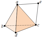
This comprises of four 2-simplices, eight 1-simplices and five 0-simplices. The boundary maps are given as above, e.g. $\partial_2([a, c, d]) = [c,d] - [a,d] + [a,c],$ $\partial_1([a,e]) = [e] - [a]$ and $\partial_0([d]) = 0.$ Now it suffices to obtain the homology groups from the sequence $\mathbb{Z}^4 \to \mathbb{Z}^8 \to \mathbb{Z}^5 \to 0$ which is left as an exercise for the reader.

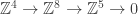
In general, expressing a topological object as a simplicial complex can be a rather tedious affair, for the vertices of each simplex must be distinct, and two distinct simplices cannot be represented by the same tuple of vertices. E.g. in the case of a torus, one possibility is the following:

which has 18 faces, 27 edges and 9 vertices. Hence, simplicial homology can be quite a hassle to compute by hand, but on the plus side one can easily write a program to compute it. Also, note that simplicial homology is a special case of cellular homology (one where all cells are simplices).

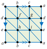
Exercise. What’s wrong with the following simplicial complex for the torus?

Answer (highlight to read) : the 1-simplices [a, c] and [a, b] are duplicated. E.g. [a, b] appears twice for the two edges at the bottom of the square.

Betti Numbers and Euler Characteristic

One can obtain the Euler characteristic of M from its Betti numbers:

Theorem. For any object M, we have:

$\chi(M) = \sum_{i\ge 0} (-1)^i b_i(M).$

Proof

We know from linear algebra that for any linear map T : V → W, we have dim(ker(T)) + dim(im(T)) = dim(V). Hence for each i, we have

$\dim(\text{ker}(\partial_i)) + \dim(\text{im}(\partial_i)) = \dim (\mathbb{R}^{S_i})=|S_i|.$

And since $b_i(M) = \dim(\text{ker}(\partial_i)) - \dim(\text{im}(\partial_{i+1}))$ , we get

$\begin{aligned}\sum_i (-1)^i b_i(M) &= \sum_i (-1)^i\dim(\text{ker}(\partial_i)) - (-1)^i\sum_i\dim(\text{im}(\partial_{i+1}))\\ &=\sum_i (-1)^i \dim(\text{ker} (\partial_i)) + \sum_i (-1)^{i+1}\dim( \text{im}(\partial_{i+1})) \\ &=\sum_i (-1)^i [\dim(\text{ker} (\partial_i)) + \dim(\text{im}(\partial_i))] \\ &= \sum_i (-1)^i |S_i| =\chi(M)\end{aligned}$

as desired. ♦

Mayer-Vietoris Sequence

Suppose $X = M\cup N$ . Recall that the principle of inclusion and exclusion allows us to compute the Euler characteristics of X from those of M, N and M ∩ N. The question is: what about Betti numbers and homology groups? We would very much like to say $b_m(X) = b_m(M) + b_m(N) - b_m(M\cap N)$ but we would be lying if we did. Instead, we have the extended exact sequence:

$\begin{aligned}\ldots &\longrightarrow H_m(M\cap N) \longrightarrow H_m(M) \oplus H_m(N) \longrightarrow H_m(M\cup N) \\ &\longrightarrow H_{m-1}(M\cap N) \longrightarrow H_{m-1}(M) \oplus H_{m-1}(N) \longrightarrow H_{m-1}(M\cup N) \ldots \end{aligned}$

[ Note: an exact sequence of abelian groups is a sequence of maps as above such that for any two consecutive maps $A \stackrel {f}\to B \stackrel{g}\to C,$ we have $\text{ker}(g) = \text{im}(f).$ Also, the direct sum $\oplus$ of two groups is simply their product. ]

Let’s explain the various maps. First, pick a cellular decomposition of M and of N; then find a decomposition of X which is a common refinement of both. The inclusion $M\hookrightarrow M\cup N$ then maps chains of M to those of $M\cup N.$ Clearly, if an m-chain D of M satisfies ∂D = 0, so does its image in $M\cup N.$ Furthermore, if the chain D is of the form ∂E for some (m+1)-chain E, then the image D’ of D in $M\cup N$ is of the form ∂E’, where E’ is the image of E in $M\cup N.$ Hence the inclusion $i_M :M\hookrightarrow M\cup N$ induces a map of homology groups:

${i_M}_* :H_m(M) \to H_m(M\cup N)$ and similarly ${i_N}_* : H_m(N) \to H_m(M\cup N).$

[ Note: even though $i_M$ and $i_N$ are injective, in general ${i_M}_*$ and ${i_N}_*$ are not. ] Likewise, the inclusions $j_M : M\cap N \hookrightarrow M$ and $j_N : M\cap N\hookrightarrow N$ induce ${j_M}_* : H_m(M\cap N) \to H_m(M)$ and ${j_N}_* : H_m(M\cap N) \to H_m(N).$ Now we define:

$H_m(M\cap N) \to H_m(M) \oplus H_m(N)$ as the map $[D] \mapsto ({j_M}_*([D]), -{j_N}_*([D]))$ ,
$H_m(M) \oplus H_m(N) \to H_m(M\cup N)$ as the map $[D] \mapsto {i_M}_*([D]) + {i_N}_*([D]).$

The map left of interest is the boundary map:

$H_m(M\cup N) \to H_{m-1}(M\cap N).$

For that, suppose we have an m-chain D of $M\cup N$ such that ∂D=0. Write it as a sum of m-chains D’+D”, where D’, D” are chains of M, N respectively. Now since ∂D’ = -∂D” is an (m-1)-chain in M as well as in N, it must be an (m-1)-chain in M ∩ N; this gives rise to the map $H_m(M\cup N) \to H_{m-1}(M\cap N).$ The boundary map is also denoted ∂, which may cause some confusion since the same symbol was earlier used to for a map taking m-chains of M to (m-1)-chains of M.

[ For the conscientious reader, the map is well-defined because

∂(∂D’) = 0 so we can take the class of ∂D’ in M ∩ N;
if we replace D by D+∂E, we can write E as a sum of (m+1)-chains E’+E”, where E’, E” are chains of M, N respectively, so D’ is replaced by D’+∂E’ which gives ∂D’ = ∂(D’+∂E’) = ∂D’;
if we pick a different D = D₁‘ + D₂“, then D₁‘–D’ = D”–D₂“ is a chain in M ∩ N, and thus ∂D₁‘ = ∂(D₁‘–D’) + ∂D’ has the same image as ∂D’ modulo im(∂) in M ∩ N. ]

Example

Let consider the 3-sphere $S^3 = \{(x,y,z,t) \in \mathbb{R}^4 : x^2+y^2 + z^2 + t^2 = 1\}.$ This is the union of

$M = \{(x,y,z,t) \in S^3 : t\ge 0\}$ and $N = \{(x,y,z,t) \in S^3 : t\le 0\}$

with intersection $M\cap N = \{(x,y,z,0) \in \mathbb{R}^4 : x^2 + y^2 + z^2 = 1\}.$ The long exact sequence above thus gives (together with $H_4 = 0$ since we’re dealing with two or three-dimensional objects here):

$\begin{aligned} 0 &\to H_3(M\cap N) \to H_3(M)\oplus H_3(N) \to H_3(S^3)\\ &\to H_2(M\cap N) \to H_2(M)\oplus H_2(N) \to H_2(S^3) \\ &\to H_1(M\cap N) \to H_1(M)\oplus H_1(N) \to H_1(S^3) \\ &\to H_0(M\cap N) \to H_0(M)\oplus H_0(N) \to H_0(S^3) \to 0.\end{aligned}$

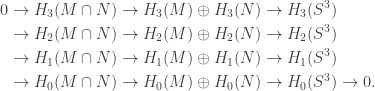
Since M and N are homeomorphic to the solid ball $\{(x,y,z) : x^2+y^2+z^2 \le 1\}$ and hence the full 3-simplex on [0, 1, 2, 3], it is easy to check that they have trivial homology in dimensions ≥ 1. On the other hand, M ∩ N is homeomorphic to the surface of a cube so we get:

$H_3(S^3) \cong H_2(M\cap N) \cong \mathbb{Z}, \ H_2(S^3) \cong H_1(M\cap N) = 0$

and $H_1(S^3) =0$ since it’s easy to check that $H_0(M\cap N)\to H_0(M) \oplus H_0(N)$ is injective.

2 Responses to From Euler Characteristics to Cohomology (II)

Osama Ghani says:

June 29, 2016 at 11:22 am

Hi there! Just wanted to ask about the definition of chains. Here you use formal linear combinations of simplices as a chain, but in Calculus on Manifolds by Spivak, he uses formal linear combinations of (what he calls) singular n-cubes, which are maps from [0,1]^n –> R^s. I know that you should be able to integrate on both kinds of chains simply, but does one offer any advantage over the other? Why is there a difference?

- limsup says:
  
  June 30, 2016 at 1:52 am
  
  The difference lies in singular or simplicial homology. Spivak is talking about singular homology while I’m talking about simplicial.
  
  Roughly, in singular homology you can prove things but can’t really compute; in simplicial homology you can compute but can’t prove much.The tough part is to show that the two are equal on a huge class of topological spaces (e.g. CW-complexes).