Continuing our discussion of modular representation theory, we will now discuss block theory. Previously, we saw that in any ring R, there is at most one way to write  where
where  is a set of orthogonal and centrally primitive idempotents. If such an expression exists, the
  are called block idempotents of R. For example, block idempotents exist when R is artinian.
We need the following refinement:
Lemma. Let be block idempotents of R. Suppose  where the
  are orthogonal central idempotents. Then there exists a unique map
  such that:
Note: if  the sum is zero
Thus after a suitable renumbering of terms, we have:

Proof
For each we have  , where
  are orthogonal central idempotents. Since is centrally primitive, we must have
  for some unique j and
  for all k≠j. The map
  then gives
  and
and  for all
  And so
 ♦
♦
Decomposition of R-Modules
Let M be an R-module and suppose  where the are block idempotents of R. Then
- Indeed,
 since each
- On the other hand, if
 then we have
  and thus
Furthermore, since commutes with every r∈R,  is in fact an R-submodule. The central idempotent acts as the identity on
  and zero on
  for j≠i. One can thus imagine:

where each  is an
is an  -module.
Block Idempotents of Semisimple R
Recall that a semisimple ring R is isomorphic to  for some division ring
  where
where  is the n × n matrix ring with entries in D. Since each matrix ring is a simple ring, we immediately obtain the central idempotents: for i=1,…,m, corresponds to the element whose component in
  is the identity matrix, and whose component in
  is the zero matrix.
As a module over itself, R is a direct sum of the spaces of column vectors, so  where
where  runs through a complete collection of simple R-modules, and the component
  gives the maximal decomposition
  as a direct sum of ideals.
In particular, this holds for the group ring K[G]. We have:
![K[G] = \oplus V^{\dim_K V}](https://s0.wp.com/latex.php?latex=K%5BG%5D+%3D+%5Coplus+V%5E%7B%5Cdim_K+V%7D&bg=ffffff&fg=333333&s=0&c=20201002) , where the direct sum is over all simple V.
, where the direct sum is over all simple V.
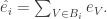
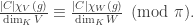
Lemma. The block idempotent for  is given by the following formula:

where  is the character of V.
Proof
Fix V; it suffices to show that  induces the identity map on
  and zero on all other components. Now the coefficients of are constant over each conjugancy class, so
 ![e_V\in Z(K[G])](https://s0.wp.com/latex.php?latex=e_V%5Cin+Z%28K%5BG%5D%29&bg=ffffff&fg=333333&s=0&c=20201002) and is K[G]-linear. If W is simple, induces a scalar map on it, say
and is K[G]-linear. If W is simple, induces a scalar map on it, say  To compute
  we take the trace:

But  and so the above sum is
  Thus
Thus  as desired. ♦

Block Idempotents of R[G]
Since k[G] is artinian, block idempotents are guaranteed to exist. Furthermore these can be lifted to block idempotents of R[G], which is a nice result since R[G] is not artinian.
Lemma. Suppose  are orthogonal central idempotents of Z(k[G]). Then we can find orthogonal central idempotents
  of R[G] such that
Proof
The proof is conceptually similar to an earlier lemma. The main step is to show:
Claim: if S is a commutative ring with ideal I such that  , then any orthogonal idempotents
  summing to 1 can be lifted to orthogonal idempotents
  summing to 1.
[ If we can show this, then idempotents ![e_i \in Z((R/\pi)[G])](https://s0.wp.com/latex.php?latex=e_i+%5Cin+Z%28%28R%2F%5Cpi%29%5BG%5D%29&bg=ffffff&fg=333333&s=0&c=20201002) can be lifted to
can be lifted to ![Z((R/\pi^2)[G]](https://s0.wp.com/latex.php?latex=Z%28%28R%2F%5Cpi%5E2%29%5BG%5D&bg=ffffff&fg=333333&s=0&c=20201002) , and in turn to
, and in turn to ![Z((R/\pi^4)[G]](https://s0.wp.com/latex.php?latex=Z%28%28R%2F%5Cpi%5E4%29%5BG%5D&bg=ffffff&fg=333333&s=0&c=20201002) etc. Since R is complete, this gives idempotents in Z(R[G]). ]
etc. Since R is complete, this gives idempotents in Z(R[G]). ]
Proof of Claim.
Pick any  such that
  . Thus:

As in the earlier proof, let  and this gives
  Also
Also  for all i≠j since it is divisible by
  (since S is commutative). Finally, we claim that
  Indeed, from the factorisation
  we obtain:

where the first equality follows from  and the second follows from
  for i≠j. Note that
  so
so  Thus
Thus  is zero. ♦
Conversely, if ![\hat{e_i}\in R[G]](https://s0.wp.com/latex.php?latex=%5Chat%7Be_i%7D%5Cin+R%5BG%5D&bg=ffffff&fg=333333&s=0&c=20201002) are orthogonal central idempotents summing to 1, then so are their images
are orthogonal central idempotents summing to 1, then so are their images ![e_i \in k[G].](https://s0.wp.com/latex.php?latex=e_i+%5Cin+k%5BG%5D.&bg=ffffff&fg=333333&s=0&c=20201002) Finally, we have:
Finally, we have:
Lemma. If ![\hat{e}, \hat{e}'\in R[G]](https://s0.wp.com/latex.php?latex=%5Chat%7Be%7D%2C+%5Chat%7Be%7D%27%5Cin+R%5BG%5D&bg=ffffff&fg=333333&s=0&c=20201002) are central idempotents with the same image in k[G], then they are equal.
are central idempotents with the same image in k[G], then they are equal.
Proof.
Let  , which is a central idempotent in πR[G]. But
 ![\hat f \in \pi^m R[G] \implies \hat f = \hat{f}^2\in \pi^{2m} R[G]](https://s0.wp.com/latex.php?latex=%5Chat+f+%5Cin+%5Cpi%5Em+R%5BG%5D+%5Cimplies+%5Chat+f+%3D+%5Chat%7Bf%7D%5E2%5Cin+%5Cpi%5E%7B2m%7D+R%5BG%5D&bg=ffffff&fg=333333&s=0&c=20201002) so we must have
so we must have  and so
  ♦
♦
Thus, we have shown:
Summary.
There is a 1-1 correspondence between:
- orthogonal central idempotents of k[G] summing to 1, and
- orthogonal central idempotents of R[G] summing to 1.
In particular, block idempotents for k[G] lift to those for R[G]:
![1 = e_1 + e_2 + \ldots + e_r,\ (e_i \in k[G]) \ \mapsto 1 = \hat{e_1} + \hat{e_2} + \ldots + \hat{e_r},\ (\hat{e_i} \in R[G]).](https://s0.wp.com/latex.php?latex=1+%3D+e_1+%2B+e_2+%2B+%5Cldots+%2B+e_r%2C%5C+%28e_i+%5Cin+k%5BG%5D%29+%5C+%5Cmapsto+1+%3D+%5Chat%7Be_1%7D+%2B+%5Chat%7Be_2%7D+%2B+%5Cldots+%2B+%5Chat%7Be_r%7D%2C%5C+%28%5Chat%7Be_i%7D+%5Cin+R%5BG%5D%29.&bg=ffffff&fg=333333&s=0&c=20201002)
Taking each ![\hat{e_i} \in K[G]](https://s0.wp.com/latex.php?latex=%5Chat%7Be_i%7D+%5Cin+K%5BG%5D&bg=ffffff&fg=333333&s=0&c=20201002) , we can write it as a sum of the block idempotents of K[G]. Thus, we can partition the set of simple K[G]-modules as a disjoint union
, we can write it as a sum of the block idempotents of K[G]. Thus, we can partition the set of simple K[G]-modules as a disjoint union  , one for each
  , such that:
For convenience, we also denote by  where χ is the character of V. This gives the formula
Example: S3.
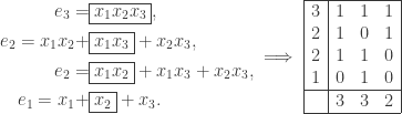
Let’s compute the central idempotents for K[S3] using the above formula. Let a = (1,2) + (2,3) + (3,1) and b = (1,2,3) + (1,3,2). We recover the example at the end of the previous article:
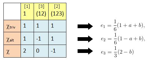
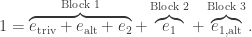
Now let’s consider the case p=2. We have  as block idempotents of R[G] (and also of k[G], after reduction mod 2), so the blocks are {e1, e2}, {e3}. For p=3, {e1, e2, e3} all belong to the same block.
If M is an indecomposable k[G]-module, then  and thus there is exactly one i for which
  , and
, and  for all j≠i. As a result, the basis elements
 ![[P] \in P_k(G)](https://s0.wp.com/latex.php?latex=%5BP%5D+%5Cin+P_k%28G%29&bg=ffffff&fg=333333&s=0&c=20201002) and
and ![[M] \in R_k(G)](https://s0.wp.com/latex.php?latex=%5BM%5D+%5Cin+R_k%28G%29&bg=ffffff&fg=333333&s=0&c=20201002) can be classified into blocks, where P (resp. M) belongs to block if and only if
can be classified into blocks, where P (resp. M) belongs to block if and only if  (resp.
  ). Note that if P belongs to block ei, then the idempotent ei acts as the identity on eiP. The same holds for M.
Similarly, for a simple K[G]-module V, there is a unique i for which  In summary, we can think of a block as a collection of:
- indecomposable finitely-generated projective k[G]-modules P;
- simple k[G]-modules M;
- simple K[G]-modules V.
Lemma. Suppose basis elements ![[P]\in P_k(G), [V]\in R_K(G)](https://s0.wp.com/latex.php?latex=%5BP%5D%5Cin+P_k%28G%29%2C+%5BV%5D%5Cin+R_K%28G%29&bg=ffffff&fg=333333&s=0&c=20201002) belong to distinct blocks ei and ej, where i≠j. Then the matrix entry of
belong to distinct blocks ei and ej, where i≠j. Then the matrix entry of  corresponding to [P], [V] is zero.
Proof
Indeed, we have  and
and 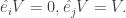 If
If ![[\hat P] \in P_R(G)](https://s0.wp.com/latex.php?latex=%5B%5Chat+P%5D+%5Cin+P_R%28G%29&bg=ffffff&fg=333333&s=0&c=20201002) is the lift of [P], we have
is the lift of [P], we have  and thus
  since
since  is an indecomposable R[G]-module. Hence
  and we must have
  for any irreducible component W of
  This shows that V cannot be a component of ♦
Corollary. Let ![[P] \in P_k(G), [M] \in R_k(G), [V]\in R_K(G)](https://s0.wp.com/latex.php?latex=%5BP%5D+%5Cin+P_k%28G%29%2C+%5BM%5D+%5Cin+R_k%28G%29%2C+%5BV%5D%5Cin+R_K%28G%29&bg=ffffff&fg=333333&s=0&c=20201002) be basis elements.
be basis elements.
- If [M] and [V] belong to different blocks, the matrix entry of
 is zero.
- If [P] and [V] belong to different blocks, the matrix entry of
 is zero.
Proof
The first statement follows from the fact that the matrix for d is the transpose of that for e; the second statement follows from c = de. ♦
Thus, the matrices for  can be broken up as block matrices, one for each block idempotent of k[G].
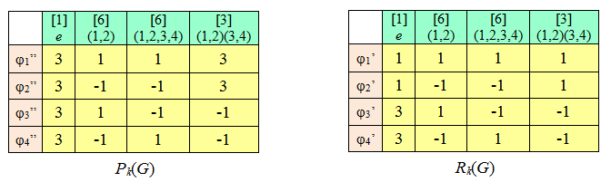
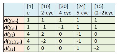
Example: S4.
The character table of S4 gives us: letting a = (sum of 2-cycles), b = (sum of 3-cycles), c = (sum of 4-cycles), d = (sum of (2+2)-cycles), the central idempotents of K[S4] are:

For p = 2, all five simple characters belong to the same block. For p = 3, we have:
Finally, we can check when two characters lie within the same block. First, we need the following lemma:
Lemma. Let R be a commutative k-algebra of finite dimension over k and be its block idempotents. Then any k-algebra homomorphism  is uniquely determined by the image of the block idempotents
Proof
Corresponding to the block idempotents, write  as a product of commutative k-algebras. Since is artinian,
  is semisimple and hence a product of matrix algebras. Since has no idempotent except 0 and 1, itself is a matrix algebra, i.e. for some division ring D/k. But R is commutative, so n=1 and D is a field extension k’ of k.
On the other hand, let  Since
Since  and the
  are orthogonal idempotents, exactly one
  is a k-algebra homomorphism while the remaining
  are zero maps for j≠i. Now
  must factor through the nilpotent ideal
  and so it is determined by
  which is either the zero map or the identity, depending on whether
  is 0 or 1. ♦
Theorem. Let V, W be simple K[G]-modules; the following are equivalent.
- V and W are in the same block.
- For any conjugancy class C⊆G and g∈C, we have:
Note
In the course of the proof, we will see that  for any simple V, so the congruence is well-defined.
Proof
Step 1. For each simple V, we will define a ring homomorphism ![\lambda_V : Z(K[G]) \to K.](https://s0.wp.com/latex.php?latex=%5Clambda_V+%3A+Z%28K%5BG%5D%29+%5Cto+K.&bg=ffffff&fg=333333&s=0&c=20201002)
Given any conjugancy class C⊆G, define  as a K-linear map V→V. Since
  commutes with all g∈G, it is a K[G]-linear map V→V. But V is simple, hence such a map is a scalar; thus we get a ring homomorphism
Step 2. Show that  is the LHS of the congruence and that this lies in R.
Taking the trace of  , we get:

So 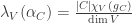 for any representative
  To prove that this lies in R, recall that we can pick an R-lattice M⊂V which is an R[G]-module. Thus
  Picking a basis for M, we have
Step 3. Compute  where
where  is the K[G] block idempotent for W.
Let us rewrite

and so 
Step 4. Complete the proof.
Since  , step 3 tells us V and W belong to the same block
  if and only if
  for all i. But this value is either 0 or 1, so it holds if and only if
 for all i.
On the other hand, ![\lambda_V(Z(R[G])) \subseteq R](https://s0.wp.com/latex.php?latex=%5Clambda_V%28Z%28R%5BG%5D%29%29+%5Csubseteq+R&bg=ffffff&fg=333333&s=0&c=20201002) so we also obtain a ring homomorphism
so we also obtain a ring homomorphism ![\lambda_V : Z(R[G]) \to R.](https://s0.wp.com/latex.php?latex=%5Clambda_V+%3A+Z%28R%5BG%5D%29+%5Cto+R.&bg=ffffff&fg=333333&s=0&c=20201002) Reduction mod π then gives us a k-algebra homomorphism
Reduction mod π then gives us a k-algebra homomorphism ![\lambda_V' : Z(k[G]) \to k.](https://s0.wp.com/latex.php?latex=%5Clambda_V%27+%3A+Z%28k%5BG%5D%29+%5Cto+k.&bg=ffffff&fg=333333&s=0&c=20201002) By the above, V and W belong to the same block if and only if
By the above, V and W belong to the same block if and only if  for all i. Since Z(k[G]) is a commutative k-algebra of finite dimension over k, the above lemma says this holds if and only if
 ![\lambda_V' = \lambda_W' : Z(k[G]) \to k](https://s0.wp.com/latex.php?latex=%5Clambda_V%27+%3D+%5Clambda_W%27+%3A+Z%28k%5BG%5D%29+%5Cto+k&bg=ffffff&fg=333333&s=0&c=20201002) which is equivalent to
which is equivalent to  for all C. ♦
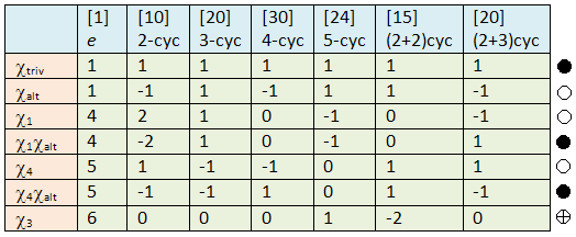
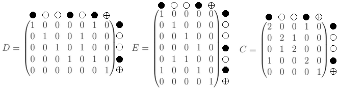
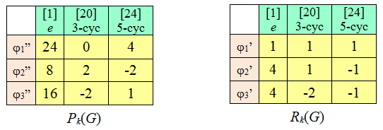
Example: S5.
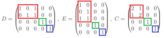
Modular 2, the blocks of the character table are labeled by the circles on the right:
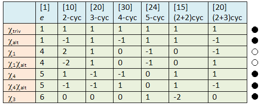
The corresponding matrices are:
Modular 3, the table becomes:

The corresponding matrices are:


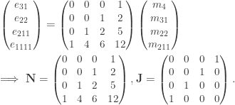
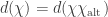
is any partition, we define:


is the number of matrices
with non-negative integer entries such that
for each j and
for each i.


is a free commutative ring, we can define a graded ring homomorphism


is an involution, i.e.
is the identity on


-basis of
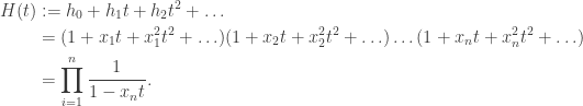
:
as a free commutative ring; the isomorphism preserves the grading, where


![h_{n+1}, h_{n+2}, \ldots \in \Lambda_n = \mathbb{Z}[h_1, \ldots, h_n],](https://s0.wp.com/latex.php?latex=h_%7Bn%2B1%7D%2C+h_%7Bn%2B2%7D%2C+%5Cldots+%5Cin+%5CLambda_n+%3D+%5Cmathbb%7BZ%7D%5Bh_1%2C+%5Cldots%2C+h_n%5D%2C&bg=ffffff&fg=333333&s=0&c=20201002)


 and write
  for the largest
  for which
  . If
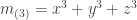
. If  For example if
  , then:
 ;
; ;
; .
. is the partition obtained by flipping the Young diagram about the main diagonal.
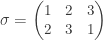
 so it helps to have an ordering on the set of all partitions of d. The lexicographical order (or dictionary order) on the set
  is given as follows:
  if and only if there is an
 if for each i we have
 We have the following.
 , we have
 . We first claim that, for each
  , we have:
 is the largest value for which
  ; equivalently,
  is the largest value for which
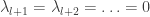
  The claim can be readily seen from the diagram below:
 Let
Let  . We have two cases.
 , then this sum is at most
  since there are more non-negative terms in the sum.
 , the sum is still at most
  are negative.
 which gives:
 ; replacing
  by their transposes we get the reverse implication. ♦
 and the transpose gives
  . On the other hand

 , the monomial
  vanishes. Now, we write the above expression vectorially.

 , the matrix must be:
 Removing the first row and dropping trailing zeros in
  the number of remaining columns is exactly
  so the second row must be filled with all 1’s. And so on. ♦
 , if
, if  then
then 
 is a binary matrix whose row sums are
  and column sums are
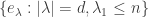
  Erase the 0’s and replace the 1’s in the matrix by consecutive 1, 2, …, d, where
  E.g. if
  and
and  , pick:
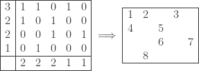
![M_S = \left[\begin{matrix} 1 & 2 & 3 \\ 4 & 5 \\6 & 7 \\8 \end{matrix}\right] \qquad M_T = \left[\begin{matrix} 1 & 2 & 5 & 3 & 7\\ 4 & 8 & 6\end{matrix}\right].](https://s0.wp.com/latex.php?latex=M_S+%3D+%5Cleft%5B%5Cbegin%7Bmatrix%7D+1+%26+2+%26+3+%5C%5C+4+%26+5+%5C%5C6+%26+7+%5C%5C8+%5Cend%7Bmatrix%7D%5Cright%5D+%5Cqquad+M_T+%3D+%5Cleft%5B%5Cbegin%7Bmatrix%7D+1+%26+2+%26+5+%26+3+%26+7%5C%5C+4+%26+8+%26+6%5Cend%7Bmatrix%7D%5Cright%5D.&bg=ffffff&fg=333333&s=0&c=20201002)
 and
and  have shapes
  respectively, i.e. there are
  terms in row i of
  By construction, if an element occurs in row i of
  then it must occur in row i or above in
 be the permutation matrix which switches
  The prior two lemmas show that
  is upper-triangular, with all 1’s on the main diagonal. Hence
  is invertible over the integers, and so is
  .
.


![\mathbb{Z}[x_1, \ldots, x_n]](https://s0.wp.com/latex.php?latex=%5Cmathbb%7BZ%7D%5Bx_1%2C+%5Cldots%2C+x_n%5D&bg=ffffff&fg=333333&s=0&c=20201002) of integer polynomials. The symmetric group
of integer polynomials. The symmetric group  acts on it by permuting the variables; specifically,
  takes:
 takes
takes  to
to  . Denote the ring of symmetric polynomials by:
![\Lambda_n:= \mathbb{Z}[x_1, \ldots, x_n]^{S_n}.](https://s0.wp.com/latex.php?latex=%5CLambda_n%3A%3D+%5Cmathbb%7BZ%7D%5Bx_1%2C+%5Cldots%2C+x_n%5D%5E%7BS_n%7D.&bg=ffffff&fg=333333&s=0&c=20201002)

 , a basis is given by:

 be the symmetric polynomial obtained by summing all terms of the form:
 , and
, and  .
. parts.
 . A basis of
  is given by:
 instead of
  . However, if the subscripts involve variables, we will include the commas for clarity.

 . Note that since
  , we can take as many terms as we want by increasing
  without affecting
  For example, when
 (here,
  where
where  denotes the sum of all
  for various
 with
with  In the remaining of this article, we will describe a more systematic method of computation.
 . Consider the expression
 with
with 
 For that, we need to find the number of binary matrices with column sums
  and row sum
  As expected, we get 5 solutions:
 and attempt to find the coefficient of
  E.g. suppose
  We wish to expand:

 by multiplying terms from
  ,
,  , etc. ♦
 In the definition of
  , then the monomial
  since it would involve more than n variables. For example, if
  and
and  , then the above expansion gives
  since
since  One can verify this directly by expanding
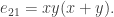
 and now
 as a linear combination of the monomial symmetric polynomials:


 ) is an idempotent if and only if f is a projection, i.e. M = ker(f) ⊕ im(f) and f : M→M projects onto im(f). Indeed ⇐ is obvious, and conversely if f is idempotent, we have:
 as a direct sum of left ideals, and
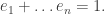
 , write
  with
with  Then each xi is idempotent since
  and each
  since Ij is a left module. Since R is the direct sum of Ij‘s we have
  for all j≠i and
  for all i. Hence the
  are orthogonal idempotents.
 since 1 lies in the RHS. On the other hand, an element of
  can be written as
  Then
Then  since the ei‘s are orthogonal. Similarly,
  for all i and thus
 with
with  We need to show
 we have
 write
write  where we have
  from what we just proved. Since
  for all j≠i and so
 Clearly
  with
with  and this is the unique representation. ♦
 then
then  is the direct sum of two non-zero left modules.
 then
then  so we do have a direct sum on the RHS.
 in the RHS, we have

 where
where  as R-modules but they are distinct left ideals of R.

![K[S_3]](https://s0.wp.com/latex.php?latex=K%5BS_3%5D&bg=ffffff&fg=333333&s=0&c=20201002) is semisimple and we have the following orthogonal idempotents:
is semisimple and we have the following orthogonal idempotents:
![e_C :=(\sum_{g\in C} g) \in R[G]](https://s0.wp.com/latex.php?latex=e_C+%3A%3D%28%5Csum_%7Bg%5Cin+C%7D+g%29+%5Cin+R%5BG%5D&bg=ffffff&fg=333333&s=0&c=20201002) where C ⊆ G is a conjugancy class.
where C ⊆ G is a conjugancy class. where
where  ; this lies in the centre iff gα = αg for all g∈G. Multiplying gives
 or equivalently for all g, x,
  ♦
♦![Z(K[G]) = K\otimes_R Z(R[G]).](https://s0.wp.com/latex.php?latex=Z%28K%5BG%5D%29+%3D+K%5Cotimes_R+Z%28R%5BG%5D%29.&bg=ffffff&fg=333333&s=0&c=20201002)
 as a product of rings;
 as a sum of orthogonal central idempotents.
 since
since  is a two-sided ideal. Now
  and
and  and since
 are orthogonal central idempotents. The prior correspondence gives
  which is a two-sided ideal since
 and
and  is a set of centrally primitive central idempotents which are orthogonal, then r=s and there is a permutation σ of {1,…,r} such that
  for all i.
 are distinct: indeed if e is orthogonal to itself, then
  Same goes for
 Since
Since  is centrally primitive and
  are orthogonal central idempotent:
 for some unique i and all remaining terms are zero. Likewise, for this i, we have
  for some unique k. So we have
  and since
  we must have j=k and so
  Since
Since  the result follows. ♦
![\mathbf{Q}[S_3].](https://s0.wp.com/latex.php?latex=%5Cmathbf%7BQ%7D%5BS_3%5D.&bg=ffffff&fg=333333&s=0&c=20201002) Note that its centre is spanned by 1, a := (1,2)+(1,3)+(2,3) and b := (1,2,3)+(1,3,2). These satisfy
Note that its centre is spanned by 1, a := (1,2)+(1,3)+(2,3) and b := (1,2,3)+(1,3,2). These satisfy

![Z(\mathbf{Q}[S_3]) \cong \mathbf{Q} \times \mathbf{Q} \times \mathbf{Q}](https://s0.wp.com/latex.php?latex=Z%28%5Cmathbf%7BQ%7D%5BS_3%5D%29+%5Ccong+%5Cmathbf%7BQ%7D+%5Ctimes+%5Cmathbf%7BQ%7D+%5Ctimes+%5Cmathbf%7BQ%7D&bg=ffffff&fg=333333&s=0&c=20201002) of rings. Since this decomposition is clearly maximal, the above three idempotents are all centrally primitive. Note that the first term is centrally primitive but not primitive since
of rings. Since this decomposition is clearly maximal, the above three idempotents are all centrally primitive. Note that the first term is centrally primitive but not primitive since
 be the modular characters of the simple k[G]-modules; they form a basis of
 be those of the projective indecomposable k[G]-modules; they form a basis of
 , the number of p-regular conjugancy classes of G.
 and
and  form a dual basis under the inner product
  so that
 be the standard irreducible characters of K[G], so they form an orthonormal basis of
 satisfies: for each
  the function
  is zero on the p-singular conjugancy classes of G.
 is the transpose of d and is injective.
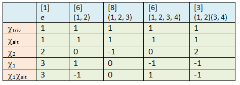
 , we leave only the columns for e and (1,2,3), since the remaining conjugancy classes are 2-singular. Immediately, we obtain some linear relations:
 ;
; ;
; and since the image is abelian, it factors through the commutator
 ![[S_n, S_n] = A_n](https://s0.wp.com/latex.php?latex=%5BS_n%2C+S_n%5D+%3D+A_n&bg=ffffff&fg=333333&s=0&c=20201002) and we obtain
and we obtain  So we are left with the trivial and alternating representations. ♦
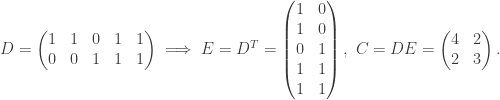
 and
and 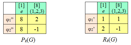
 as expected. E.g.
 and
and  take all the 2-singular classes to 0.
 and
and  in the decomposition of φ, and the multiplicty of
  and
and  among its composition factors.
 and
and  are simple since they’re of dimension 1. Next, we have
  It remains to see if
  and
and  are simple. Consider
  If it weren’t simple it must contain a submodule of dimension 1, which we saw is either
 where
where  Since
Since  this means both eigenvalues for (1,2,3,4) are -1, and so those for its square (1,3)(2,4) are +1. But this contradicts
 where
where  so both eigenvalues for (a, b) are +1. This means all elements of S4 have both eigenvalues equal to +1, which is absurd.

 for any character χ so we are left with 4 rows. Next
  so we are left with
  which are clearly linearly independent. Writing them as linear combinations of simple modular characters:
 we are further reduced to 12 possibilities (corresponding to their values at e, the 3-cycle and 5-cycle):
 for any g, this immediately removes the first 7 possibilities. Next
  is invalid since for
  we must have 3 fifth roots of unity summing up to -2, which is impossible. So we’re left with two choices. It turns out
  is the right choice, which we shall show below.
 contains the trivial representation.
  is found in the representation
  where V is a 4-dimensional representation given by:
 acts on V by permuting the coordinates. Another way of expressing this is:
  where
where  and g∈G acts on
  by taking
  Now
Now  is spanned by
  where multiplication commutes. A basis of W is given by
  and
and
 , which is G-invariant. Note that this vector is non-zero (simplify via
  ).
). for all 1≤i≤j≤4. Note that
  and
and  and so we see that f is G-equivariant, where G acts trivially on k. Note that f(X)=0 so we have at least two copies of the trivial representation among the composition factors.

 and
and 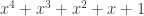 respectively. Lifting the roots of unity to K gives us
  for the first case and
  for the second, where
  and
and  so the values are
  and
and  respectively.
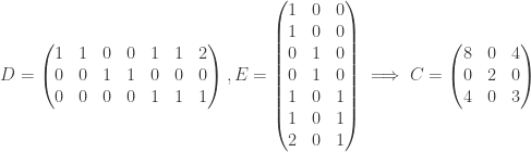


 is even if
  Note that this holds if and only if φ is zero on the odd permutations: 2-cyc and 4-cyc (we’re ignoring the (2+3)cyc column for modular characters mod 3). Since φ is simple if and only if
  is, we see that
  are either all even, or exactly one of them is even. The former case is impossible since that would imply
  all take the same values for 2-cyc and 4-cyc. Hence, we may assume
  and that
  is even.
 we would have φ(e) = 3 and φ(5-cyc) = -2, which is impossible since we cannot have 3 fifth roots of unity summing to -2.
 is impossible.
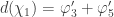 . This means
  is even, it must be
  Hence we have
 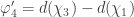 which takes 2-cyc to -2. Hence
  takes 2-cyc to +2 and so it must be the identity (contradiction).
 The latter would imply
  where
where 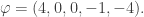 Hence the eigenvalues for (2+2)cyc are all -1 and since its order is coprime to p=3, the matrix for (2+2)cyc is –I. But then we have (1,3)(2,4)·(1,2,3,4,5) = (1,4,5,3,2) and we cannot have both
  and
and 
 and we have:
 for which
 for all basis elements
 ![x = [P] \in P_k(G)](https://s0.wp.com/latex.php?latex=x+%3D+%5BP%5D+%5Cin+P_k%28G%29&bg=ffffff&fg=333333&s=0&c=20201002) and
and ![y = [M] \in R_K(G)](https://s0.wp.com/latex.php?latex=y+%3D+%5BM%5D+%5Cin+R_K%28G%29&bg=ffffff&fg=333333&s=0&c=20201002) , i.e. P is projective indecomposable and M is simple. As seen
, i.e. P is projective indecomposable and M is simple. As seen ![e(x) = [K\otimes_R Q],](https://s0.wp.com/latex.php?latex=e%28x%29+%3D+%5BK%5Cotimes_R+Q%5D%2C&bg=ffffff&fg=333333&s=0&c=20201002) where
where 
 for some R[G]-module N, free over R, so that d(y) = N/πN.
![\dim_k \text{Hom}_{k[G]}(Q/\pi Q, N/\pi N) = \dim_K \text{Hom}_{K[G]}(K\otimes_R Q, K\otimes_R N).](https://s0.wp.com/latex.php?latex=%5Cdim_k+%5Ctext%7BHom%7D_%7Bk%5BG%5D%7D%28Q%2F%5Cpi+Q%2C+N%2F%5Cpi+N%29+%3D+%5Cdim_K+%5Ctext%7BHom%7D_%7BK%5BG%5D%7D%28K%5Cotimes_R+Q%2C+K%5Cotimes_R+N%29.&bg=ffffff&fg=333333&s=0&c=20201002)
![X:= \text{Hom}_{R[G]}(Q, N) = \text{Hom}_R(Q, N)^G](https://s0.wp.com/latex.php?latex=X%3A%3D+%5Ctext%7BHom%7D_%7BR%5BG%5D%7D%28Q%2C+N%29+%3D+%5Ctext%7BHom%7D_R%28Q%2C+N%29%5EG&bg=ffffff&fg=333333&s=0&c=20201002) ; this is R-free since it is a submodule of a free R-module. Our desired result would follow if we could show:
; this is R-free since it is a submodule of a free R-module. Our desired result would follow if we could show:![X/\pi X \cong \text{Hom}_{k[G]}(Q/\pi Q, N/\pi N), \qquad K\otimes_R X \cong \text{Hom}_{K[G]}(K\otimes_R Q, K\otimes_R N).](https://s0.wp.com/latex.php?latex=X%2F%5Cpi+X+%5Ccong+%5Ctext%7BHom%7D_%7Bk%5BG%5D%7D%28Q%2F%5Cpi+Q%2C+N%2F%5Cpi+N%29%2C+%5Cqquad+K%5Cotimes_R+X+%5Ccong+%5Ctext%7BHom%7D_%7BK%5BG%5D%7D%28K%5Cotimes_R+Q%2C+K%5Cotimes_R+N%29.&bg=ffffff&fg=333333&s=0&c=20201002)
![Q\oplus Q' \cong R[G]^n](https://s0.wp.com/latex.php?latex=Q%5Coplus+Q%27+%5Ccong+R%5BG%5D%5En&bg=ffffff&fg=333333&s=0&c=20201002) for some R[G]-module Q’ and n>0. Since direct sum commutes with tensor product, it suffices to prove the above two isomorphisms for
for some R[G]-module Q’ and n>0. Since direct sum commutes with tensor product, it suffices to prove the above two isomorphisms for ![Q = R[G].](https://s0.wp.com/latex.php?latex=Q+%3D+R%5BG%5D.&bg=ffffff&fg=333333&s=0&c=20201002) Now this is obvious since in this case, X=N, and we have
Now this is obvious since in this case, X=N, and we have![\begin{aligned}\text{Hom}_{k[G]}(Q/\pi Q, N/\pi N) &= \text{Hom}_{k[G]}(k[G], N/\pi N) \cong N/\pi N = X/\pi X\\ \text{Hom}_{K[G]}(K\otimes_R Q, K\otimes_R N) &= \text{Hom}_{K[G]}(K[G], K\otimes_R N) = K\otimes_R N = X\otimes_R N\end{aligned}](https://s0.wp.com/latex.php?latex=%5Cbegin%7Baligned%7D%5Ctext%7BHom%7D_%7Bk%5BG%5D%7D%28Q%2F%5Cpi+Q%2C+N%2F%5Cpi+N%29+%26%3D+%5Ctext%7BHom%7D_%7Bk%5BG%5D%7D%28k%5BG%5D%2C+N%2F%5Cpi+N%29+%5Ccong+N%2F%5Cpi+N+%3D+X%2F%5Cpi+X%5C%5C+%5Ctext%7BHom%7D_%7BK%5BG%5D%7D%28K%5Cotimes_R+Q%2C+K%5Cotimes_R+N%29+%26%3D+%5Ctext%7BHom%7D_%7BK%5BG%5D%7D%28K%5BG%5D%2C+K%5Cotimes_R+N%29+%3D+K%5Cotimes_R+N+%3D+X%5Cotimes_R+N%5Cend%7Baligned%7D&bg=ffffff&fg=333333&s=0&c=20201002)
 so e(x) = 0. But a basis of
 ![e([P]) \in R_K(G)](https://s0.wp.com/latex.php?latex=e%28%5BP%5D%29+%5Cin+R_K%28G%29&bg=ffffff&fg=333333&s=0&c=20201002) are linearly independent.
are linearly independent. where
where  its trace as a K-linear map. Since K[G] is semisimple, standard character theory says
  uniquely determines M. Now,
  where
where  does not lead to a satisfactory theory. The better approach is to lift the character to a function G→R.
 Note that this is a union of conjugancy classes.
 Consider the k-linear map
  Let r be the order of g; since r|m, k contains all the eigenvalues of g, denoted

 This is easily seen by taking a k-basis of N, then extending to give a k-basis of M. Hence
 ![\varphi_M =: \varphi_{[M]}](https://s0.wp.com/latex.php?latex=%5Cvarphi_M+%3D%3A+%5Cvarphi_%7B%5BM%5D%7D&bg=ffffff&fg=333333&s=0&c=20201002) is independent of our choice of [M] in the Grothendieck group
is independent of our choice of [M] in the Grothendieck group  Then
Then 
 for all p-regular g. [ Note that the tensor product is over k and not k[G]. ]
 and the second one gives a modular character
  From the definition, we have:

 and
and  These clearly give the same values for all p-regular g. Furthermore, the following shows that
  when g is p-singular.
![R[G] = R[T]/\left< T^{m\cdot p^r} - 1\right>](https://s0.wp.com/latex.php?latex=R%5BG%5D+%3D+R%5BT%5D%2F%5Cleft%3C+T%5E%7Bm%5Ccdot+p%5Er%7D+-+1%5Cright%3E&bg=ffffff&fg=333333&s=0&c=20201002)
![k[G] = k[T]/\left<T^{m\cdot p^r}-1\right> \cong \oplus_i k[T]/\left<(T - \zeta_i)^{p^r}\right>](https://s0.wp.com/latex.php?latex=k%5BG%5D+%3D+k%5BT%5D%2F%5Cleft%3CT%5E%7Bm%5Ccdot+p%5Er%7D-1%5Cright%3E+%5Ccong+%5Coplus_i+k%5BT%5D%2F%5Cleft%3C%28T+-+%5Czeta_i%29%5E%7Bp%5Er%7D%5Cright%3E&bg=ffffff&fg=333333&s=0&c=20201002)
 is of codimension 1. The corresponding R[G]-module is then
 ![M_i=R[T]/\left<T^{p^r} - \zeta_i'\right>.](https://s0.wp.com/latex.php?latex=M_i%3DR%5BT%5D%2F%5Cleft%3CT%5E%7Bp%5Er%7D+-+%5Czeta_i%27%5Cright%3E.&bg=ffffff&fg=333333&s=0&c=20201002) Since r>0, multiplication by T has trace zero in each
Since r>0, multiplication by T has trace zero in each  which maps to
  ♦
♦
![\left< P, M\right>_k := \dim_k \text{Hom}_{k[G]}(P, M)](https://s0.wp.com/latex.php?latex=%5Cleft%3C+P%2C+M%5Cright%3E_k+%3A%3D+%5Cdim_k+%5Ctext%7BHom%7D_%7Bk%5BG%5D%7D%28P%2C+M%29&bg=ffffff&fg=333333&s=0&c=20201002)
 and
and  for any k[G]-module N.
 For the dual we pick
 ![k\cdot f \subseteq k[G]^*](https://s0.wp.com/latex.php?latex=k%5Ccdot+f+%5Csubseteq+k%5BG%5D%5E%2A&bg=ffffff&fg=333333&s=0&c=20201002) where f : k[G]→k takes e to 1 and all other g to 0; and for the tensor product, we pick
where f : k[G]→k takes e to 1 and all other g to 0; and for the tensor product, we pick ![k\cdot e\otimes_k N \subseteq k[G]\otimes_k N.](https://s0.wp.com/latex.php?latex=k%5Ccdot+e%5Cotimes_k+N+%5Csubseteq+k%5BG%5D%5Cotimes_k+N.&bg=ffffff&fg=333333&s=0&c=20201002) ♦
♦
 is a free R-module and
 is a R-submodule of a free R-module, so it must be R-free. Now write
 ![\tilde Q \oplus \tilde M \cong R[G]^n](https://s0.wp.com/latex.php?latex=%5Ctilde+Q+%5Coplus+%5Ctilde+M+%5Ccong+R%5BG%5D%5En&bg=ffffff&fg=333333&s=0&c=20201002) for some R[G]-module
for some R[G]-module  and so
  On the other hand, we have
 ![Q\oplus M\cong k[G]^n](https://s0.wp.com/latex.php?latex=Q%5Coplus+M%5Ccong+k%5BG%5D%5En&bg=ffffff&fg=333333&s=0&c=20201002) so
so  Comparing terms then gives
  ]
] is R[G]-projective, its character
  vanishes on the p-singular elements and the above equals:
 is said to be a p-regular class function. An inner product is defined on the space of all such functions:
![[P]\in P_k(G)](https://s0.wp.com/latex.php?latex=%5BP%5D%5Cin+P_k%28G%29&bg=ffffff&fg=333333&s=0&c=20201002) and
and ![[M]\in R_k(G)](https://s0.wp.com/latex.php?latex=%5BM%5D%5Cin+R_k%28G%29&bg=ffffff&fg=333333&s=0&c=20201002) for projective indecomposable P and simple M give rise to dual bases
for projective indecomposable P and simple M give rise to dual bases  and
and  under the above inner product.
 is injective. Hence
  is the number of p-regular conjugancy classes of G.
 then taking the inner product with
  for each simple M gives:
 is surjective but the proof of this is rather involved and we may revisit this again some day.
 and
and  So if
So if  is an exact sequence of k[G]-modules, then so is:
 which is bi-additive. Since tensor product is associative, we obtain a ring structure on
  we see that
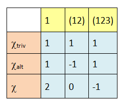
 and
and  So the modular character tables for
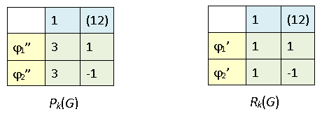
 and
and  and both vanish at the 3-cycle as expected. Furthermore one can verify by direct computation that
 ![\mathbf{Z}[T]/\left<T^2 - 1\right>](https://s0.wp.com/latex.php?latex=%5Cmathbf%7BZ%7D%5BT%5D%2F%5Cleft%3CT%5E2+-+1%5Cright%3E&bg=ffffff&fg=333333&s=0&c=20201002) where {1, T} maps to
where {1, T} maps to  respectively. Then
 , a two-sided ideal of K[G]. If K[G] = I⊕J for some left ideal J of K[G], then dim J = 1 so it is spanned by, say,
  . Since αg is a scalar multiple of α for each g∈G, all the bg‘s must be equal to some b∈K. But this means
  lies in I since its sum of coefficients is
  ♦
♦ be the
  are free abelian groups, with the following bases,
  : [M] for simple modules M.
 , taking [P] to [P/JP]; this corresponds to identity matrix (under the above bases).
![[M] = [N] \in R_k(G)](https://s0.wp.com/latex.php?latex=%5BM%5D+%3D+%5BN%5D+%5Cin+R_k%28G%29&bg=ffffff&fg=333333&s=0&c=20201002) , then M and N have identical composition factors but M and N may not be isomorphic. On the other hand, if
, then M and N have identical composition factors but M and N may not be isomorphic. On the other hand, if ![[M] = [N] \in P_k(G)](https://s0.wp.com/latex.php?latex=%5BM%5D+%3D+%5BN%5D+%5Cin+P_k%28G%29&bg=ffffff&fg=333333&s=0&c=20201002) , then the decomposition factors of M and N are the same and thus M ≅ N.
, then the decomposition factors of M and N are the same and thus M ≅ N. taking
 ![[M], [N] \mapsto \dim_K \text{Hom}_{K[G]}(M, N)](https://s0.wp.com/latex.php?latex=%5BM%5D%2C+%5BN%5D+%5Cmapsto+%5Cdim_K+%5Ctext%7BHom%7D_%7BK%5BG%5D%7D%28M%2C+N%29&bg=ffffff&fg=333333&s=0&c=20201002) is a bi-additive map. The above basis for
is a bi-additive map. The above basis for  taking
 ![[P], [M] \mapsto \dim_k \text{Hom}_{k[G]}(P, M)](https://s0.wp.com/latex.php?latex=%5BP%5D%2C+%5BM%5D+%5Cmapsto+%5Cdim_k+%5Ctext%7BHom%7D_%7Bk%5BG%5D%7D%28P%2C+M%29&bg=ffffff&fg=333333&s=0&c=20201002) is a bi-additive map. The given bases for
is a bi-additive map. The given bases for  if P/JP ≅ M. ]
 . The class of this module
 ![[N/\pi N] \in R_k(G)](https://s0.wp.com/latex.php?latex=%5BN%2F%5Cpi+N%5D+%5Cin+R_k%28G%29&bg=ffffff&fg=333333&s=0&c=20201002) depends only on M.
depends only on M. as K-vector spaces. Now let
  which is also a free R-module since it is torsion-free, and has a basis spanning M. Thus
  Since N is G-invariant it is an R[G]-module.
 are R[G]-modules such that
  Replacing
  by a scalar multiple (this does not affect
 ![[N_1]](https://s0.wp.com/latex.php?latex=%5BN_1%5D&bg=ffffff&fg=333333&s=0&c=20201002) ), we may assume
), we may assume  Now for each
  we have
  for some r; since
  for some r>0.
![[N_1/\pi N_1]= [N_2/\pi N_2]](https://s0.wp.com/latex.php?latex=%5BN_1%2F%5Cpi+N_1%5D%3D+%5BN_2%2F%5Cpi+N_2%5D&bg=ffffff&fg=333333&s=0&c=20201002) in
in  ; we have an exact sequence of k[G]-modules:
 we have
 ![[N_2/\pi N_2] = [N_1/\pi N_1]](https://s0.wp.com/latex.php?latex=%5BN_2%2F%5Cpi+N_2%5D+%3D+%5BN_1%2F%5Cpi+N_1%5D&bg=ffffff&fg=333333&s=0&c=20201002) in the group
in the group  we have:
![[N_1/\pi N_1] = [N_3/\pi N_3] = [N_2/\pi N_2]](https://s0.wp.com/latex.php?latex=%5BN_1%2F%5Cpi+N_1%5D+%3D+%5BN_3%2F%5Cpi+N_3%5D+%3D+%5BN_2%2F%5Cpi+N_2%5D&bg=ffffff&fg=333333&s=0&c=20201002) and we’re done. ♦
and we’re done. ♦![[M]\in R_K(G)](https://s0.wp.com/latex.php?latex=%5BM%5D%5Cin+R_K%28G%29&bg=ffffff&fg=333333&s=0&c=20201002) pick an R[G]-module N such that
pick an R[G]-module N such that ![d([M]) := [N/\pi N].](https://s0.wp.com/latex.php?latex=d%28%5BM%5D%29+%3A%3D+%5BN%2F%5Cpi+N%5D.&bg=ffffff&fg=333333&s=0&c=20201002)
 splits as M ≅ M’ ⊕ M”; picking modules N’ and N” for M’ and M” via the above proposition, N := N’ ⊕ N” also satisfies the proposition for M, and we obtain d([M]) = d([M’]) + d([M”]) as desired, so d is well-defined.

 ,
, ![[P] \mapsto [P/\pi P]](https://s0.wp.com/latex.php?latex=%5BP%5D+%5Cmapsto+%5BP%2F%5Cpi+P%5D&bg=ffffff&fg=333333&s=0&c=20201002) where
where  is the Grothendieck group of finitely-generated projective R[G]-modules. [ Warning: since R[G] is not artinian, we have to avoid using results from the previous two articles. ] Note that Ψ is well-defined:
![P\oplus Q\cong R[G]^n](https://s0.wp.com/latex.php?latex=P%5Coplus+Q%5Ccong+R%5BG%5D%5En&bg=ffffff&fg=333333&s=0&c=20201002) for some n so
for some n so ![(P/\pi P)\oplus (Q/\pi Q)\cong k[G]^n](https://s0.wp.com/latex.php?latex=%28P%2F%5Cpi+P%29%5Coplus+%28Q%2F%5Cpi+Q%29%5Ccong+k%5BG%5D%5En&bg=ffffff&fg=333333&s=0&c=20201002) and so P/πP is projective over k[G].
and so P/πP is projective over k[G]. as k[G]-modules, then
  as R[G]-modules.
 be an isomorphism of k[G]-modules. Since P is projective, the map
  lifts to a map
  of R[G]-modules such that the reduction of f1 mod π is f0. To show that f1 is bijective, it suffices to show it is an isomorphism of R-modules. But P, Q are finite R-free since they are projective over R[G] and thus torsion-free. So we only need to show that det(f1) is invertible in R, i.e. ≠0 modulo π. But det(f1) mod π = det(f0) ≠ 0. ♦
![k[G] = N\oplus N'.](https://s0.wp.com/latex.php?latex=k%5BG%5D+%3D+N%5Coplus+N%27.&bg=ffffff&fg=333333&s=0&c=20201002) The image of 1∈k[G] in N then gives an idempotent x∈N (i.e. x2=x). We wish to lift x to an idempotent y∈R[G] such that x = y mod π.
The image of 1∈k[G] in N then gives an idempotent x∈N (i.e. x2=x). We wish to lift x to an idempotent y∈R[G] such that x = y mod π.![S := R[G]/\pi^2 R[G]](https://s0.wp.com/latex.php?latex=S+%3A%3D+R%5BG%5D%2F%5Cpi%5E2+R%5BG%5D&bg=ffffff&fg=333333&s=0&c=20201002) with ideal
with ideal ![I:=\pi R[G]/\pi^2 R[G].](https://s0.wp.com/latex.php?latex=I%3A%3D%5Cpi+R%5BG%5D%2F%5Cpi%5E2+R%5BG%5D.&bg=ffffff&fg=333333&s=0&c=20201002) This satisfies I2 = 0 and S/I ≅ k[G] so by the claim, x lifts to an idempotent y’∈S.
This satisfies I2 = 0 and S/I ≅ k[G] so by the claim, x lifts to an idempotent y’∈S.![S' := R[G]/\pi^3 R[G]](https://s0.wp.com/latex.php?latex=S%27+%3A%3D+R%5BG%5D%2F%5Cpi%5E3+R%5BG%5D&bg=ffffff&fg=333333&s=0&c=20201002) with ideal
with ideal ![I' := \pi^2 R[G]/\pi^3 R[G].](https://s0.wp.com/latex.php?latex=I%27+%3A%3D+%5Cpi%5E2+R%5BG%5D%2F%5Cpi%5E3+R%5BG%5D.&bg=ffffff&fg=333333&s=0&c=20201002) Again
Again  and S’/I’ ≅ S so y’ lifts to an idempotent y”∈S’. Repeating this process, since R is a complete discrete valuation ring, we obtain an idempotent y∈R[G] such that x = y mod π.
![[M]\in P_R(G)](https://s0.wp.com/latex.php?latex=%5BM%5D%5Cin+P_R%28G%29&bg=ffffff&fg=333333&s=0&c=20201002) to
to ![[K\otimes_R M] \in R_K(G).](https://s0.wp.com/latex.php?latex=%5BK%5Cotimes_R+M%5D+%5Cin+R_K%28G%29.&bg=ffffff&fg=333333&s=0&c=20201002)
![[Q] = \psi^{-1}([P]) \in P_R(G)](https://s0.wp.com/latex.php?latex=%5BQ%5D+%3D+%5Cpsi%5E%7B-1%7D%28%5BP%5D%29+%5Cin+P_R%28G%29&bg=ffffff&fg=333333&s=0&c=20201002) so that
so that  Then the element e([P]) is given by
 ![[K\otimes_R Q] \in R_K(G).](https://s0.wp.com/latex.php?latex=%5BK%5Cotimes_R+Q%5D+%5Cin+R_K%28G%29.&bg=ffffff&fg=333333&s=0&c=20201002) To obtain
To obtain ![d([K\otimes_R Q])](https://s0.wp.com/latex.php?latex=d%28%5BK%5Cotimes_R+Q%5D%29&bg=ffffff&fg=333333&s=0&c=20201002) we recover Q as the R[G]-module in the definition of d and take:
we recover Q as the R[G]-module in the definition of d and take: ![d([K\otimes_R Q]) = [Q/\pi Q] = [P] \in R_k(G)](https://s0.wp.com/latex.php?latex=d%28%5BK%5Cotimes_R+Q%5D%29+%3D+%5BQ%2F%5Cpi+Q%5D+%3D+%5BP%5D+%5Cin+R_k%28G%29&bg=ffffff&fg=333333&s=0&c=20201002) as desired.
as desired.
 is idempotent, and we obtain:
![\begin{aligned} W := k[G]x &= \left< e + (1,2), (1,3) + (1,2,3), (2,3)+(1,3,2)\right>, \\ W' :=k[G](1-x) &= \left< e - (1,2), (1,3) - (1,2,3), (2,3) - (1,3,2)\right>.\end{aligned}](https://s0.wp.com/latex.php?latex=%5Cbegin%7Baligned%7D+W+%3A%3D+k%5BG%5Dx+%26%3D+%5Cleft%3C+e+%2B+%281%2C2%29%2C+%281%2C3%29+%2B+%281%2C2%2C3%29%2C+%282%2C3%29%2B%281%2C3%2C2%29%5Cright%3E%2C+%5C%5C+W%27+%3A%3Dk%5BG%5D%281-x%29+%26%3D+%5Cleft%3C+e+-+%281%2C2%29%2C+%281%2C3%29+-+%281%2C2%2C3%29%2C+%282%2C3%29+-+%281%2C3%2C2%29%5Cright%3E.%5Cend%7Baligned%7D&bg=ffffff&fg=333333&s=0&c=20201002)
![\begin{aligned} K[G]x &= \left< e + (1,2), (1,3) + (1,2,3), (2,3)+(1,3,2)\right>, \\ K[G](1-x) &= \left< e - (1,2), (1,3) - (1,2,3), (2,3) - (1,3,2)\right>.\end{aligned}](https://s0.wp.com/latex.php?latex=%5Cbegin%7Baligned%7D+K%5BG%5Dx+%26%3D+%5Cleft%3C+e+%2B+%281%2C2%29%2C+%281%2C3%29+%2B+%281%2C2%2C3%29%2C+%282%2C3%29%2B%281%2C3%2C2%29%5Cright%3E%2C+%5C%5C+K%5BG%5D%281-x%29+%26%3D+%5Cleft%3C+e+-+%281%2C2%29%2C+%281%2C3%29+-+%281%2C2%2C3%29%2C+%282%2C3%29+-+%281%2C3%2C2%29%5Cright%3E.%5Cend%7Baligned%7D&bg=ffffff&fg=333333&s=0&c=20201002)
 and
and  So the matrix for e is:
![[P] = [Q_1] + \ldots + [Q_r]](https://s0.wp.com/latex.php?latex=%5BP%5D+%3D+%5BQ_1%5D+%2B+%5Cldots+%2B+%5BQ_r%5D&bg=ffffff&fg=333333&s=0&c=20201002) in P(R) for projective modules
in P(R) for projective modules  then
then 
![f_R([P]) := [P/JP]](https://s0.wp.com/latex.php?latex=f_R%28%5BP%5D%29+%3A%3D+%5BP%2FJP%5D&bg=ffffff&fg=333333&s=0&c=20201002) , where J := J(R) is the
, where J := J(R) is the  gives a bijection between projective indecomposable modules and simple modules. Since P(R) is freely generated by the projective indecomposable modules while K(R) is freely generated by the simple modules, we have:
![f_R : P(R) \to K(R), [P] \mapsto [P/JP]](https://s0.wp.com/latex.php?latex=f_R+%3A+P%28R%29+%5Cto+K%28R%29%2C+%5BP%5D+%5Cmapsto+%5BP%2FJP%5D&bg=ffffff&fg=333333&s=0&c=20201002) is a group isomorphism.
is a group isomorphism. can be represented by a matrix with integer entries; let’s compute this for a simple example.
 Denoting the consecutive factors by A, B, C, we see that in K(R), we have [I] = [A], [J] = [A]+[B], [K] = [A]+[B]+[C], so the matrix is:
![R=\begin{pmatrix} \mathbf{Q} & \mathbf{Q}(\sqrt 2) & \mathbf{Q}(\sqrt[4]2)\\ 0 & \mathbf{Q}(\sqrt 2) & \mathbf{Q}(\sqrt[4]2) \\ 0 & 0 & \mathbf{Q}(\sqrt[4]2)\end{pmatrix}](https://s0.wp.com/latex.php?latex=R%3D%5Cbegin%7Bpmatrix%7D+%5Cmathbf%7BQ%7D+%26+%5Cmathbf%7BQ%7D%28%5Csqrt+2%29+%26+%5Cmathbf%7BQ%7D%28%5Csqrt%5B4%5D2%29%5C%5C+0+%26+%5Cmathbf%7BQ%7D%28%5Csqrt+2%29+%26+%5Cmathbf%7BQ%7D%28%5Csqrt%5B4%5D2%29+%5C%5C+0+%26+0+%26+%5Cmathbf%7BQ%7D%28%5Csqrt%5B4%5D2%29%5Cend%7Bpmatrix%7D&bg=ffffff&fg=333333&s=0&c=20201002)
![\left<-, -\right> : P(R) \times K(R) \to K(\mathbf{Z}), \qquad \left<[P], [M]\right> :=[\text{Hom}_R(P, M)].](https://s0.wp.com/latex.php?latex=%5Cleft%3C-%2C+-%5Cright%3E+%3A+P%28R%29+%5Ctimes+K%28R%29+%5Cto+K%28%5Cmathbf%7BZ%7D%29%2C+%5Cqquad+%5Cleft%3C%5BP%5D%2C+%5BM%5D%5Cright%3E+%3A%3D%5B%5Ctext%7BHom%7D_R%28P%2C+M%29%5D.&bg=ffffff&fg=333333&s=0&c=20201002)
![[\text{Hom}_R(P,M)] =[\text{Hom}_R(Q, M)]+ [\text{Hom}_R(Q', M)].](https://s0.wp.com/latex.php?latex=%5B%5Ctext%7BHom%7D_R%28P%2CM%29%5D+%3D%5B%5Ctext%7BHom%7D_R%28Q%2C+M%29%5D%2B+%5B%5Ctext%7BHom%7D_R%28Q%27%2C+M%29%5D.&bg=ffffff&fg=333333&s=0&c=20201002)

![[\text{Hom}_R(P, M)] = [\text{Hom}_R(P, M')] + [\text{Hom}_R(P, M'')]](https://s0.wp.com/latex.php?latex=%5B%5Ctext%7BHom%7D_R%28P%2C+M%29%5D+%3D+%5B%5Ctext%7BHom%7D_R%28P%2C+M%27%29%5D+%2B+%5B%5Ctext%7BHom%7D_R%28P%2C+M%27%27%29%5D&bg=ffffff&fg=333333&s=0&c=20201002) as well.
as well. , we get an exact sequence
 is a collection of projective modules, then so is
 is identified with N→N”.

 , where J := J(R) is the
  But then
  so repeating this gives us
  for all n. Since R is artinian,
  Each
Each  is projective since it is a direct summand of R. Among all
  one of them is non-zero and is surjective (since M is simple). By the above
  is simple; since it surjects onto M, we get an isomorphism. ♦
 for some n>0. By the above lemma,
  since P is projective. Now apply the Krull-Schmidt theorem: since P is indecomposable, it must be a direct summand of R. ♦