Polynomials and Representations III

Complete Symmetric Polynomials

Corresponding to the elementary symmetric polynomial, we define the complete symmetric polynomials in $\Lambda_n$ to be:

$h_0=1, \qquad h_k = \sum_{1 \le i_1 \le i_2 \le \ldots \le i_k \le n} x_{i_1} x_{i_2} \ldots x_{i_k} = \sum_{a_1 + \ldots + a_n = k} x_1^{a_1} x_2^{a_2} \ldots x_n^{a_n}.$

For example when $n=3$ , we have:

$\begin{aligned} h_3 &= x_1^3 + x_2^3 + x_3^3 + x_1^2 x_2 + x_1 x_2^2 + x_2^2 x_3 + x_2 x_3^2 + x_1^2 x_3 + x_1 x_3^2 + x_1 x_2 x_3\\ &= m_3 + m_{21} + m_{111}. \end{aligned}$

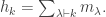
Thus, written as a sum of monomial symmetric polynomials, we have $h_k = \sum_{\lambda\vdash k} m_\lambda.$ Note that while the elementary symmetric polynomials only go up to $e_n$ , the complete symmetric polynomial $h_k$ is defined for all $k.$ Finally, we define as before:

Definition. If $\lambda$ is any partition, we define:

$h_\lambda := h_{\lambda_1} h_{\lambda_2} \ldots h_{\lambda_l},$

assuming $\lambda_{l+1} = 0.$

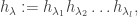
Proceeding as before, let us write $h_\lambda$ as in terms of the monomial symmetric polynomials $m_\mu.$

Theorem. We have:

$h_\lambda = \sum_{\mu} M_{\lambda\mu} m_\mu$

where $M_{\lambda\mu}$ is the number of matrices $a_{ij}$ with non-negative integer entries such that $\sum_i a_{ij} = \lambda_j$ for each j and $\sum_j a_{ij} = \mu_i$ for each i.

Proof

The proof proceeds as earlier. Let us take the example of $\lambda = (2, 2, 2)$ and $\mu = (3, 2, 1)$ . Multiplying $h_2 h_2 h_2$ , we pick the following terms to obtain the product $x_1^3 x_2^2 x_3.$

$\begin{aligned} h_2 &= \boxed{x_1^2} + x_2^2 + \ldots + x_1 x_2 + x_1 x_3 + x_2 x_3 + \ldots \\ h_2 &= x_1^2 + x_2^2 + \ldots + \boxed{x_1 x_2} + x_1 x_3 + x_2 x_3 + \ldots \\ h_2 &= x_1^2 + x_2^2 + \ldots + x_1 x_2 + x_1 x_3 + \boxed{x_2 x_3} + \ldots \\ \end{aligned} \implies \begin{array}{|c|ccc|}\hline 2 & 2 & 0 & 0 \\2 & 1 & 1 & 0 \\2 & 0 & 1 & 1 \\ \hline & 3 & 2 & 1 \\ \hline\end{array}.$

Thus each matrix corresponds to a way of obtaining $x^\mu := \prod_i x_i^{\mu_i}$ by taking terms from $h_{\lambda_1}, h_{\lambda_2},$ etc. ♦

Example

Suppose we take partitions $\lambda = (2, 2)$ , $\mu = (2, 1, 1)$ . Then $M_{\lambda\mu} = 4$ since we have the following matrices:

four_integer_matrices

Exercise

Compute $M_{\lambda\mu}$ for all partitions $\lambda, \mu$ of 4. Calculate the resulting 5 × 5 matrix, by ordering the partitions reverse lexicographically.

blue-lin

Generating Functions

The elementary symmetric polynomials satisfy the following:

$e_0 + e_1 t + e_2 t^2 + \ldots + e_n t^n = (1 + x_1 t)(1 + x_2 t) \ldots (1 + x_n t).$

Thus their generating function is given by $E(t) := \prod_{i=1}^n (1 + x_i t).$ Next, the generating function for the $h_k$’s is given by:

$\begin{aligned}H(t) &:= h_0 + h_1 t + h_2 t^2 + \ldots \\ &= (1 + x_1 t + x_1^2 t^2 + \ldots) (1 + x_2 t + x_2^2 t^2 + \ldots ) \ldots (1 + x_n t + x_n^2 t^2 + \ldots)\\ &= \prod_{i=1}^n \frac 1 {1 - x_n t}.\end{aligned}$

From $H(t)E(-t) = 1$ , we obtain the following relation:

$e_0 h_k - e_1 h_{k-1} + \ldots + (-1)^k e_k h_0 = 0, \qquad \text{ for } k=1, 2, \ldots.$

Note that $e_i = 0$ for $i > n.$

From this recurrence relation, we can express each $h_k$ as a polynomial in $e_1, \ldots, e_n$ . E.g.

$\begin{aligned} h_1 &= e_1, \\h_2 &= e_1^2 - e_2,\\h_3 &= e_1^3 - 2 e_1 e_2 + e_3,\\&\vdots\end{aligned}$

blue-lin

Duality Between e and h

From the symmetry of the recurrence relation, we can swap the h‘s and e‘s and the expressions are still correct, e.g. $e_3 = h_1^3 - 2 h_1 h_2 + h_3.$ As another example, if n=3, we have $e_4 = h_1^4 - 3h_1^2 h_2 + 2h_1 h_3 + h_2^2 - h_4 = 0.$

Definition. Since $\Lambda_n \cong \mathbb{Z}[e_1, \ldots, e_n]$ is a free commutative ring, we can define a graded ring homomorphism

$\omega: \Lambda_n \to \Lambda_n, \qquad e_i \mapsto h_i$

for $1\le i \le n.$

From what we have seen, the following comes as no surprise.

Proposition. $\omega$ is an involution, i.e. $\omega^2$ is the identity on $\Lambda_n.$

Proof.

We will prove by induction on $k$ that $w(h_k) = e_k$ for $0\le k\le n.$ For $k=0$ this is obvious; suppose $0<k\le n$ . Apply $\omega$ to the above recurrence relation; since $\omega(e_i) = h_i$ for $0\le i\le k$ we have:

$h_0 \omega(h_k) - h_1 \omega(h_{k-1}) + \ldots + (-1)^k h_k \omega(h_0) = 0.$

By induction hypothesis $\omega(h_i) = e_i$ for $i=0, \ldots, k-1$ ; since $h_0 = 1$ we have

$\omega(h_k) = h_1 e_{k-1} - h_2 e_{k-2} + \ldots + (-1)^{k-1} h_k e_0 = h_0 e_k = e_k.$

Hence $\omega^2(e_k) = e_k$ for all $k$ ; since $e_1,\ldots, e_n$ generate $\Lambda_n$ we are done. ♦

Now suppose $|\lambda| = d$ ; write $h_\lambda \in \Lambda_n^{(d)}$ as an integer linear combination of the $e_\mu$ for $|\mu| = d, \mu_1 \le n.$ Applying $\omega$ , this gives $e_\lambda$ in terms of $h_\mu$ for $|\mu| = d, \mu_1 \le n.$ In particular, we get:

Corollary. The following gives a $\mathbb{Z}$ -basis of $\Lambda_n^{(d)}$ :

$\{h_\lambda : |\lambda| = d, \lambda_1 \le n\}.$

Hence we also have $\Lambda_n \cong \mathbb{Z}[h_1, \ldots, h_n]$ as a free commutative ring; the isomorphism preserves the grading, where $\deg(h_i)=i.$

Exercise

Consider the matrix $\mathbf M = (M_{\lambda\mu}), \mathbf N = (N_{\lambda\mu})$ , where $\lambda, \mu$ run through all partitions of d. Using the involution $\omega,$ prove that

$\left(\mathbf M\mathbf N^{-1}\right)^2 = \mathbf I.$

In particular, M is invertible; this is not obvious from its definition.

Exercise

Since $h_{n+1}, h_{n+2}, \ldots \in \Lambda_n = \mathbb{Z}[h_1, \ldots, h_n],$ each $h_k$ can be uniquely expressed as a polynomial in $h_1, \ldots, h_n.$ For n=3, express $h_4, h_5$ in terms of $h_1, h_2, h_3.$