[ Background required: basic knowledge of linear algebra, e.g. the previous post. Updated on 6 Dec 2011: added graphs in Application 2, courtesy of wolframalpha.]
Those of you who already know inner products may roll your eyes at this point, but there’s really far more than what meets the eye. First, the definition:
Definition. We shall consider  , which is the set of all triplets (x, y, z) of real numbers. The inner product (or scalar product) between
  and
and  is defined to be:

[ Note: everything we say will be equally applicable to  , but it helps to keep things in perspective by looking at smaller cases. ]
The purpose of the inner product is made clear by the following theorem.
Theorem 1. Let A, B be represented by points and respectively. If O is the origin, then  is the value
  , where |l| denotes the length of a line segment l and θ is the angle between OA and OB.

Proof. It’s really simpler than you might think: just follow the following baby steps.
- Check that the dot product is symmetric (i.e. v·w = w·v for any v, w in ).
- Check that the dot product is linear in each term (v·(w + x) = (v·w) + (v·x) and v·(cw) = c(v·w) for any real c and v, w, x in ).
- From the above properties, show that 2v·w = v·v + w·w – (v–w)·(v–w).
- By Pythagoras, the RHS is
 . Now use the cosine law. ♦
Next we wish to generalise the concept of the standard basis e1 = (1,0,0), e2 = (0,1,0), e3 = (0,0,1). The key property we shall need is that they are mutually perpendicular and of length 1. From now onward, we shall sometimes call the elements of vectors. Don’t worry too much if you’re not familiar with this term.
Definitions. Thanks to the above theorem, the following definitions make sense.
- The length of a vector v is denoted by |v| = √(v·v).
- A unit vector is a vector of length 1.
- Two vectors v and w are said to be orthogonal if their inner product v·w is 0.
- A set of vectors is said to be orthonormal if (i) they are all unit vectors, and (ii) any two of them are orthogonal.
- A set of three orthonormal vectors in is called an orthonormal basis.
[ In general, any orthonormal set can be extended to an orthonormal basis, and any orthonormal basis has exactly 3 elements. We won’t prove this, but geometrically it should be obvious. Hopefully we’ll get around to abstract linear algebra, from which this will follow quite naturally. ]
Our favourite orthonormal basis is e1 = (1,0,0), e2 = (0,1,0), e3 = (0,0,1).
In general, the nice thing about an orthonormal basis is that in order to express any arbitrary vector v as a linear combination v = c1e1 + c2e2 + c3e3, there’s no need to solve a system of linear equations. Instead we just take the dot product.
Theorem 2. Let {v1, v2, v3} be an orthonormal basis. Every vector w is uniquely expressible as w = c1v1 + c2v2 + c3v3, where ci is given by ci = w·vi.
Proof. Suppose w is of the form w = c1v1 + c2v2 + c3v3. Then we apply linearity of the dot product (see proof of theorem 1) to get:

Since the vi‘s are orthonormal, the only surviving term is  . This proves the last statement, as well as uniqueness. To prove existence, let ci = w·vi and x = c1v1 + c2v2 + c3v3. We see that for i=1,2,3 we have:

so w – x is orthogonal to all three vectors {v1, v2, v3}. This contradicts the fact that we cannot have more than 3 vectors in an orthonormal basis of . ♦
[ Geometrically, the idea is to project w onto each of {v1, v2, v3} in turn to get the coefficients. ]
For example, consider the three vectors (1, 0, -2), (2, 2, 1), (4, -5, 2). They are mutually orthogonal but clearly not unit vectors. To fix that, we replace each vector v by an appropriate scalar multiple: v/|v|, so we get:
 ,
,
which is a bona fide orthonormal set. Now if we wish to write w = (1, 2, -3) as c1v1 + c2v2 + c3v3, we get:


Application 1: Cauchy-Schwartz Inequality
Square both sides of theorem 1 and obtain, for any two vectors v and w:
 .
.
Writing v = (x, y, z) and w = (a, b, c), we obtain the all-important Cauchy-Schwarz inequality:
Cauchy-Schwarz Inequality. If x, y, z, a, b, c are real numbers, then:
 .
.
Equality holds if and only if (a, b, c) and (x, y, z) are scalar multiples of each other.
Example 1.1. If a = b = c = 1/3, then we get the (root mean square) ≥ (arithmetic mean) inequality: for positive real x, y, z, we have

Example 1.2. Given that a, b, c are real numbers such that a+2b+3c = 1, find the minimum possible value of a2 + 2b2 + 3c2.
Solution. Skilfully choose the right coefficients in the Cauchy-Schwarz inequality:

to get our desired result:  . And equality holds if and only if (a, b, c) is a scalar multiple of (1, 1, 1), i.e.
  .
.
Example 1.3. Given that a, b, c, d are real numbers such that a+b+c+d = 7 and a2 + b2 + c2 + d2 = 13, find the maximum and minimum possible values of d.
Hint: [highlight start] Compare the sums a + b + c and a^2 + b^2 + c^2 using Cauchy-Schwarz inequality. Express it in terms of d. [highlight end].
Application 2: Fourier Analysis
Warning: this section is lacking in rigour, since our objective is to give the intuition behind it. It’s also rated advanced, as it’s significantly harder than the preceding text, and has quite a bit of calculus involved.
A common problem in acoustic theory is to analyse auditory waveforms. We can treat such a waveform as a periodic function  , and for convenience, we will denote the period by 2π. Now the most common functions with period 2π are:
- constant function f(x) = c;
- trigonometric functions f(x) = sin(mx) and cos(mx), m = 1, 2, … ;
It turns out any sufficiently “nice” periodic function can be approximated with these functions, i.e.

This is called the Fourier decomposition of f. The main period 2π is called the base frequency of the wave form while the higher multiples 4π, 6π, … are the harmonics. In the Fourier decomposition, one can approximate f(x) by dropping the higher harmonics, just like we can approximate a real number by taking only a certain number of decimal places.
So how does one compute the coefficients  and
and  ? For that, we consider the simple case where f is a linear combination of sin(x), sin(2x), sin(3x), i.e. we assume:
 , where
  .
.
Let V be the set of all functions  of this form. We can think of V as a vector space, similar to via the following bijection:
 .
.
So given just the waveform of f, how do we obtain a, b and c? The answer is surprisingly simple: if we take the inner product in V via:

then the functions sin(x), sin(2x), sin(3x) are orthogonal! This can be easily verified as follows: for distinct positive integers m and n, we have


However, they’re not quite orthonormal because they’re not unit vectors, Specifically, we have:
 .
.
In summary, we see that  ,
,  ,
,  form an orthonormal basis of V, under the above inner product.
Now given any function f in V, we can recover the values a, b and c by taking the inner product:
Main Theorem of Fourier Analysis
Suppose f is a 2π-periodic function such that f and df/dx are both piecewise continuous. [ A function g is piecewise continuous if  and
and  both exist for all
  . ] Then we can approximate f as a linear combination:

where  , and for n = 1, 2, 3, …, we have
  ,
,  . The above approximation means that for any real a, the RHS converges to
  . In particular, if f is continuous at x=a, then the RHS converges to f(a) for x=a.
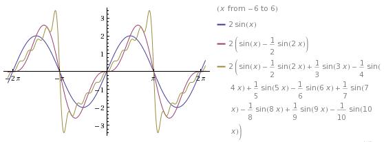
Example 2.1. Consider the function  for
for  and repeated through the real line with a period of 2π. To compute its Fourier expansion, we have:
 for any n since f(-x) = –f(x) almost everywhere (except at discrete points);
 , using integration by parts.
Thus we have  and equality holds for
  . Let’s see what the graphs of the partial sums look like.
If we substitute the value x = π/2, we obtain:

Important : at any  , both the left and right limits of f(x) at x=a must exist. So we cannot take a function like f(x) = 1/x near x=0.
Example 2.2. Take  for
for  and repeated with period 2π. Its Fourier expansion gives:
 since f(x) = f(-x) everywhere.
 .
. , for n = 1, 2, … .
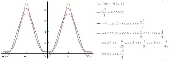
This gives  . Now equality holds on the entire interval
  since f(x) is continuous there. The graphs of the partial sums are as follows:
Substituting x=π gives:
 .
.
Simplifying gives  , which was proven by Euler via an entirely different method.
Example 2.3. This is a little astounding. Let  for , and again repeated with a period of 2π. The Fourier coefficients give:
So we can write ![e^x \sim \frac {\sinh\pi}\pi \left[ 1 + \sum_{n\ge 1} \frac{2(-1)^n}{n^2+1}\cos(nx) + \sum_{n\ge 1}\frac{2n(-1)^{n+1}}{n^2+1}\sin(nx)\right]](https://s0.wp.com/latex.php?latex=e%5Ex+%5Csim+%5Cfrac+%7B%5Csinh%5Cpi%7D%5Cpi+%5Cleft%5B+1+%2B+%5Csum_%7Bn%5Cge+1%7D+%5Cfrac%7B2%28-1%29%5En%7D%7Bn%5E2%2B1%7D%5Ccos%28nx%29+%2B+%5Csum_%7Bn%5Cge+1%7D%5Cfrac%7B2n%28-1%29%5E%7Bn%2B1%7D%7D%7Bn%5E2%2B1%7D%5Csin%28nx%29%5Cright%5D&bg=ffffff&fg=333333&s=0&c=20201002) , which holds for all . In particular, for x = 0, we get the rather mystifying identity:
, which holds for all . In particular, for x = 0, we get the rather mystifying identity:
![1 = \frac{\sinh\pi}\pi \left[ 1 - \frac{2}{1^2+1} + \frac{2}{2^2+1}-\frac{2}{3^2+1}\dots\right],](https://s0.wp.com/latex.php?latex=1+%3D+%5Cfrac%7B%5Csinh%5Cpi%7D%5Cpi+%5Cleft%5B+1+-+%5Cfrac%7B2%7D%7B1%5E2%2B1%7D+%2B+%5Cfrac%7B2%7D%7B2%5E2%2B1%7D-%5Cfrac%7B2%7D%7B3%5E2%2B1%7D%5Cdots%5Cright%5D%2C&bg=ffffff&fg=333333&s=0&c=20201002)
which you can verify numerically to some finite precision.

 . It’s clear what the corresponding building blocks of symmetric polynomials would be:
 ;
; ;
; ;
; .
.
 :
: (*)
(*) . Some of these are quite easy:
 ;
; ;
; .
. in terms of the elementary symmetric polynomials
  ,
,  ,
,  .
. . We already know how to express this in terms of P, Q and R :
 .
. . ♦
. ♦ holds in the 5-variable case. And so on. This allows us to generalise the recurrence (*) to include all Sk.
 be the sum of the k-th powers of the variables xi. Then we have:
 ;
; ;
; ;
; .
.

 and
and  . Hence
  . Next, we use the root-mean-square & arithmetic-mean inequality (a special case of


 are solutions. Upon clearing denominators and simplifying, we get a quartic equation in the form of
  . Since the degree of the polynomial is 4, its roots are precisely 4, 16, 36, 64. On the other hand, the sum of roots is the negative of the coefficient of T3, which is 84+x+y+z+w; so x+y+z+w = 36. ♦


 , then xy, xz, xw, yz, yw, zw are roots of the sextic polynomial
  .
.
 .
.
 in the expansion of
  . Once again, any symmetric polynomial in x, y, z with integer coefficients can be expressed as a polynomial in P, Q and R with integer coefficients.
 , then using the technique described in the
 ,
,  ,
,  , we obtain:
 ;
; …
… .
. , so:
, so: .
. . ♦
. ♦ and
and  . Express the polynomial
  as a polynomial in P, Q, R.
 . That’s too much to solve linearly, so we prune down the cases further by singling out one variable: x. Indeed, the degree of x in A is 4, with leading coefficient
  . So:
. So: and
and  can’t appear since they contain higher powers of x, i.e.
  ;
; only appears in
  and
and  , with respective leading terms
  and
and  . So
. So  .
. from the coefficient of
  .
. so we get


 , where T is unknown. Since x, y and z are distinct, these are precisely all the roots. Expanding the polynomial gives
  and the sum of the roots is thus given by 3s. Yet the sum of the roots is also x+y+z = s. Thus s=0 and x, y and z are roots of
  . So
. So  and other permutations. ♦

 in terms of P, Q and R.
 .
. is symmetric while
  is not symmetric.
 is also an integer (for any natural number n) although x and y themselves may not be integral: e.g.
  , y = 3 – \sqrt 2$.
 . This can be written as
  and then we use the substitution
  . So
. So  .
. for integer n and proceed to derive a recurrence relation in
  . First, suppose we fix x and y; let
  be the quadratic equation with roots x and y. Then
  and
and  . Now since x and y are both roots of that quadratic equation, we have:
 respectively, we obtain:
 . Since this holds for any x and y, we see that
  as polynomials in x and y.
 as a polynomial in P and Q with just a bit of work. Starting with
  and
and  , we have:
 ;
; ;
; ;
; .
. .
. whose roots are x and y. In other words,
  as polynomials. From the above computations, we have
  and thus
 .
. . The first case gives complex roots while the second case gives
  or
or  . ♦
. ♦ . Try it!
 . [ Note: it may not be possible to arrive at the answer via guesswork; in fact, a, b, x, y may well be irrational, but the above sums turn out to be rational. ]
 and
and  . Multiplying the two equations by
  and
and  respectively, we get:
 . Upon adding the above two equations, we get a recurrence:
 ,
,  ,
,  ,
,  . Substituting into the recurrence relation above, we obtain:
 and the final answer is:
 . ♦
. ♦ . Find the quadratic equation whose roots are
  and
and  .
. ; γ and δ are roots of the equation
  . Prove that
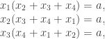
 .
. , where all vectorial values are given in boldface. One imagines this as a particle travelling along the curve such that at time t, its position is at x(t). Recall that the velocity of the particle is then given by
  which is parallel to the gradient of the curve at x(t).
 , from which it’s clear that the distance travelled by the particle during a time interval [a,b] is given by:
 parametrized via
  . The arc length of the curve from (0,0) to (1,1) is given by
  which is
  , i.e. around 1.479, which is only slightly longer than the straight line joining the two points.
 from (0,0) to (1,1).
 , find the formula of the arc-length.
 . Since regardless of parametrization,
  . Let’s calculate its parametrization by arc-length s, via the hard way. [ The easy way is via polar coordinates. ] Starting from the point (-5, 0), the arc-length to the point
  is given by:
 ,
,  , where
  . This is consistent with our intuition that the arc-length is a linear function of the angle θ.
 . Parametrize the curve by arc-length, starting from the origin (0, 0).
 and parametrize it by arc-length, starting from
  .
. is parametrized by arc-length, then
  . [ Note: if your concept is right, this should be a 2-line proof. We will need this result later. ]
 be the unit tangent vector of the curve
  , parametrized by arc-length. The curvature
  of a curve is defined by
  .
. .
. we need to show that after parametrizing by arc-length that:
 ). The RHS remains unchanged thanks to the way we
  and
and  .
. and it suffices to compute
  . To do that, note that the vector
  is parallel to the tangent of the curve at the point
  , so we can express the unit tangent vector in terms of x :
 .
. . So our definition is consistent with the earlier one. Notice that the curvature vector
  is perpendicular to tangent vector (x-axis). This always holds.
 be a curve in n-space, with components
  . Everything follows as before:
 .
. .
. is
is  , or
, or  .
. .
.
 , so the tangent vector is
  . To compute the curvature vector, we apply:
 .
. . Hence, the curvature vector is given by
  . and the curvature is 1/5. In other words, the helix has constant curvature, which is consistent with our geometric figure.
 . Compute the curvature and curvature vector at a general point on the curve.
 , where
  and
and  . Hence:
 ;
; ;
; ;
; ;
; and the scalar curvature is
  .
. where
where  . Recall that the first derivative
  tells us the gradient of the curve at a point. To be precise, at the point
  , the value
  is exactly the gradient of the curve at
  .
. . In secondary school calculus, we have little use for this value, except to determine whether a curve is a local maximum, minimum or stationary point. However, it’s quite clear on an intuitive level that
  tells us how much the curve turns at
  for different values of a: as a > 0 increases, the curve bends more and more at the origin (0,0).
 . In the general case, if we wish to define the curvature at a point, rotate and translate the curve so that the point maps to the origin and the curve is tangent to the x-axis. Now apply the previous definition.
 makes an angle of θ with the x-axis, then
  . To rotate this an angle of
  , we use the transformation

 at
at  since
since 
 and
and 
 .
. at any point is equal to
  .
. . Use this to obtain a simpler proof of 2.
 . Locate where they occur.
 where both coordinates are integers. Let P be a polygon on the cartesian plane such that every vertex is a lattice point (we call it a lattice polygon). Pick’s theorem tells us that the area of P can be computed solely by counting lattice points:
 , where i = number of lattice points in P and b = number of lattice points on the boundary of P.

 .
. , m, n not both zero, P and the translate P + (m, n) have disjoint interior. [ If they share an interior point, then P must contain a vertex of P + (m, n) which is not one of 0, v, w, v+w. ]
 (see below), the pieces do not intersect. As a result, the area is at most 1.
 . Indeed: each light at an internal point clearly contributes
  while the sum of the angles in an m-sided polygon is
  by elementary geometry.
 on the inside and
  on the outside. So the total angle is
  which corresponds to an area of 11/2.
 where
where  . Arrange them in increasing order. E.g. for N = 4, we get:
 in lowest terms, we have
  . Although not obvious at first glance, this follows directly from Pick’s theorem. Indeed, let’s draw a ray from the origin (0, 0) to the point (a, b) for each reduced fraction
  , i.e. the shaded region below:
 are consecutive in the Farey sequence. This requires the fact that the shaded region is convex. [ A region R is said to be convex if whenever points P and Q lie in R, so is the entire line segment PQ. ]
 , so the result follows.
 and sort them in ascending order. Then since the resulting shaded region is also convex, we also have
  for any consecutive reduced fractions
 be a Farey sequence of some order. Write
  in lowest terms and construct a circle on the upper-half plane which is tangent to
  and has radius
  . Then two consecutive circles are tangent.
 is expressed in lowest terms
  , m must be a multiple of p.
 .
. , … .
, … . . The sum in parenthesis simplifies to a fraction
  in lowest terms, where s is not divisible by p. Hence the sum is
  in lowest terms, so m = pr is a multiple of p. ♦
 :
: = the set of all rational numbers of the form
  .
. is said to be divisible by
  (for positive integer n) if we can find
  such that
  .
. are all elements of
 is divisible by q=7 if there is a
  such that x = 7y. What happens? Why, then every element of
  is a multiple of 7 and the definition is meaningless.
 if the difference
  is divisible by
  and
and  .
. .
. .
. .
. , then
  .
. such that
  and
and  . [ The proofs for the first 3 properties are identical to the case of integers! ]
 ;
; ;
; ;
; .
. modulo
  , where b is not divisible by p, it suffices to show
  is congruent to some integer integer mod
  for some integers r and s. Now we get
  and our job is done. ♦
 . As a tradeoff, however, now we can only talk about congruence modulo powers of p, instead of general n.
 . So we need to show
  . This is not hard:
 , the squares are all distinct (if not, then
  , so
, so  is a multiple of p and either
  or
or  is a multiple of p).
 for
for  are also distinct. (*)
 , the squares
  cover all the possible non-zero squares mod p and they’re all distinct.
 .
.![1, \frac 1 {2^2}, \frac 1 {3^2}, \dots, \frac 1 {[(p-1)/2]^2}](https://s0.wp.com/latex.php?latex=1%2C+%5Cfrac+1+%7B2%5E2%7D%2C+%5Cfrac+1+%7B3%5E2%7D%2C+%5Cdots%2C+%5Cfrac+1+%7B%5B%28p-1%29%2F2%5D%5E2%7D&bg=ffffff&fg=333333&s=0&c=20201002) are congruent to
are congruent to  modulo p, after some permutation. Hence, modulo p, our sum is congruent to
 . Define the sum:
 in lowest terms, then
  .
. for positive integer n. Find all positive integers k which are coprime to all
  in the sequence.


 .
. .
. .
. of Q is obviously Q(10) mod 10, i.e. n mod 10, and the coefficient
  of X is then given by
  etc.
etc. .
. and
and  , we have
  . So
. So  .
. which is congruent to
  .
. are unique. Then we need to prove that
  , the constant term of
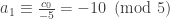
  , is unique. Substituting Q(-2) = n and Q(-5) = n, we get:
 , and
, and  (*),
(*), and subsequently every
  for all i > N. [ In mathematical lingo, we say “for all large enough i“. ]
 and
and  .
. and
and  . We obtain the following.
 . OK.
. OK. and
and  , so we have
  ,
,  . Thus
  .
. and
and  . So
. So  and
and 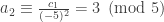 . Thus
  .
. and
and  . Hence
  and
and  and
and  .
. and
and  so we have
  and
and  . This gives
  .
. and
and  so $latex a_5 \equiv \frac{b_4}{(-2)^5} = -1 \pmod 2$ and
 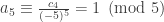 . Thus
  .
. . So we’re done.
 and
and  , so actually, all we need is the fact that bk and ck are bounded sequences. So let’s try to bound them in terms of n. In attempting to prove this, we’ve to be careful. Note that if we had replaced -2 and -5 by +2 and +5 respectively, the result clearly doesn’t hold for negative integers. So our proof must somehow distinguish between these 2 cases.
 (and same holds for (-5)-case) so induction follows.
 holds for sufficiently large |n|; specifically, n ≤ -10 suffices, for then we would have:
 .
.
 (#)
(#) and
and  . The sequence of t‘s then gives the coefficients. For the starting value of (1, 0), we get (1, 0) → (2, 1) → (2, 1) → (2, 1) … . So we get an infinite power series
  rather than a polynomial!
 for all but finitely many
  , we can list them all out. The only possibilities are:
 . So if we start from (n, n), we will always have
  , while for the second and third case, we have a – b ≡ 1, 2 (mod 3) respectively.