Linear Algebra: Inner Products

[ Background required: basic knowledge of linear algebra, e.g. the previous post. Updated on 6 Dec 2011: added graphs in Application 2, courtesy of wolframalpha.]

Those of you who already know inner products may roll your eyes at this point, but there’s really far more than what meets the eye. First, the definition:

Definition. We shall consider $\mathbb R^3$ , which is the set of all triplets (x, y, z) of real numbers. The inner product (or scalar product) between $\mathbf v = (x,y,z)$ and $\mathbf v' = (x',y',z')$ is defined to be:

$\mathbf v \cdot \mathbf v' = (x, y, z)\cdot (x',y',z') = xx' + yy' + zz' \in \mathbb R.$

[ Note: everything we say will be equally applicable to $\mathbb R^n$ , but it helps to keep things in perspective by looking at smaller cases. ]

The purpose of the inner product is made clear by the following theorem.

Theorem 1. Let A, B be represented by points $\mathbf v = (x,y,z)$ and $\mathbf v' = (x',y',z')$ respectively. If O is the origin, then $\mathbf v\cdot \mathbf v'$ is the value $|OA| \cdot |OB| \cos \theta$ , where |l| denotes the length of a line segment l and θ is the angle between OA and OB.

Proof. It’s really simpler than you might think: just follow the following baby steps.

Check that the dot product is symmetric (i.e. v·w = w·v for any v, w in $\mathbb R^3$ ).
Check that the dot product is linear in each term (v·(w + x) = (v·w) + (v·x) and v·(cw) = c(v·w) for any real c and v, w, x in $\mathbb R^3$ ).
From the above properties, show that 2v·w = v·v + w·w – (v–w)·(v–w).
By Pythagoras, the RHS is $|OA|^2+|OB|^2-|AB|^2$ . Now use the cosine law. ♦

Next we wish to generalise the concept of the standard basis e₁ = (1,0,0), e₂ = (0,1,0), e₃ = (0,0,1). The key property we shall need is that they are mutually perpendicular and of length 1. From now onward, we shall sometimes call the elements of $\mathbb R^3$ vectors. Don’t worry too much if you’re not familiar with this term.

Definitions. Thanks to the above theorem, the following definitions make sense.

The length of a vector v is denoted by |v| = √(v·v).
A unit vector is a vector of length 1.
Two vectors v and w are said to be orthogonal if their inner product v·w is 0.
A set of vectors is said to be orthonormal if (i) they are all unit vectors, and (ii) any two of them are orthogonal.
A set of three orthonormal vectors in $\mathbb R^3$ is called an orthonormal basis.

[ In general, any orthonormal set can be extended to an orthonormal basis, and any orthonormal basis has exactly 3 elements. We won’t prove this, but geometrically it should be obvious. Hopefully we’ll get around to abstract linear algebra, from which this will follow quite naturally. ]

Our favourite orthonormal basis is e₁ = (1,0,0), e₂ = (0,1,0), e₃ = (0,0,1).

In general, the nice thing about an orthonormal basis is that in order to express any arbitrary vector v as a linear combination v = c₁e₁ + c₂e₂ + c₃e₃, there’s no need to solve a system of linear equations. Instead we just take the dot product.

Theorem 2. Let {v₁, v₂, v₃} be an orthonormal basis. Every vector w is uniquely expressible as w = c₁v₁ + c₂v₂ + c₃v₃, where c_i is given by c_i = w·v_i.

Proof. Suppose w is of the form w = c₁v₁ + c₂v₂ + c₃v₃. Then we apply linearity of the dot product (see proof of theorem 1) to get:

$\mathbf w \cdot \mathbf v_i = (c_1 \mathbf v_1 + c_2\mathbf v_2 + c_3\mathbf v_3)\cdot v_i = c_1(v_1\cdot v_i) + c_2(v_2\cdot v_i) + c_3(v_3\cdot v_i).$

Since the v_i‘s are orthonormal, the only surviving term is $c_i (v_i \cdot v_i) = c_i$ . This proves the last statement, as well as uniqueness. To prove existence, let c_i = w·v_i and x = c₁v₁ + c₂v₂ + c₃v₃. We see that for i=1,2,3 we have:

$\mathbf x \cdot \mathbf v_i = (c_1\mathbf v_1 + c_2\mathbf v_2 + c_3\mathbf v_3)\cdot \mathbf v_i = c_i = \mathbf w\cdot \mathbf v_i,$

so w – x is orthogonal to all three vectors {v₁, v₂, v₃}. This contradicts the fact that we cannot have more than 3 vectors in an orthonormal basis of $\mathbb R^3$ . ♦

[ Geometrically, the idea is to project w onto each of {v₁, v₂, v₃} in turn to get the coefficients. ]

For example, consider the three vectors (1, 0, -2), (2, 2, 1), (4, -5, 2). They are mutually orthogonal but clearly not unit vectors. To fix that, we replace each vector v by an appropriate scalar multiple: v/|v|, so we get:

$\mathbf v_1 = \frac 1 {\sqrt 5} (1, 0, -2), \mathbf v_2 = \frac 1 3 (2, 2, 1), \mathbf v_3 = \frac 1 {3\sqrt 5} (4, -5, 2)$ ,

which is a bona fide orthonormal set. Now if we wish to write w = (1, 2, -3) as c₁v₁ + c₂v₂ + c₃v₃, we get:

$\mathbf w = \frac 7 {\sqrt 5} \mathbf v_1 + \mathbf v_2 - \frac 4 {\sqrt 5}\mathbf v_3.$

Application 1: Cauchy-Schwartz Inequality

Square both sides of theorem 1 and obtain, for any two vectors v and w:

$(\mathbf v\cdot \mathbf w)^2 \le |\mathbf v|^2 |\mathbf w|^2$ .

Writing v = (x, y, z) and w = (a, b, c), we obtain the all-important Cauchy-Schwarz inequality:

Cauchy-Schwarz Inequality. If x, y, z, a, b, c are real numbers, then:

$(a^2 + b^2 + c^2)(x^2 + y^2 + z^2) \ge (ax + by + cz)^2$ .

Equality holds if and only if (a, b, c) and (x, y, z) are scalar multiples of each other.

Example 1.1. If a = b = c = 1/3, then we get the (root mean square) ≥ (arithmetic mean) inequality: for positive real x, y, z, we have

$\sqrt{\frac{x^2+y^2+z^2} 3} \ge \frac {x+y+z} 3.$

Example 1.2. Given that a, b, c are real numbers such that a+2b+3c = 1, find the minimum possible value of a² + 2b² + 3c².

Solution. Skilfully choose the right coefficients in the Cauchy-Schwarz inequality:

$(a^2 + (\sqrt 2 b)^2 + (\sqrt 3 c)^2)(1^2 + ({\sqrt 2})^2 + ({\sqrt 3})^2) \ge (a + 2b + 3c)^2$

to get our desired result: 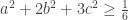$a^2 + 2b^2 + 3c^2 \ge \frac 1 6$ . And equality holds if and only if (a, b, c) is a scalar multiple of (1, 1, 1), i.e. $(a,b,c) = \pm (\frac 1 6, \frac 1 6, \frac 1 6)$ .

Example 1.3. Given that a, b, c, d are real numbers such that a+b+c+d = 7 and a² + b² + c² + d² = 13, find the maximum and minimum possible values of d.

Hint: [highlight start] Compare the sums a + b + c and a^2 + b^2 + c^2 using Cauchy-Schwarz inequality. Express it in terms of d. [highlight end].

Application 2: Fourier Analysis

Warning: this section is lacking in rigour, since our objective is to give the intuition behind it. It’s also rated advanced, as it’s significantly harder than the preceding text, and has quite a bit of calculus involved.

A common problem in acoustic theory is to analyse auditory waveforms. We can treat such a waveform as a periodic function $f:\mathbb R \to\mathbb R$ , and for convenience, we will denote the period by 2π. Now the most common functions with period 2π are:

constant function f(x) = c;
trigonometric functions f(x) = sin(mx) and cos(mx), m = 1, 2, … ;

It turns out any sufficiently “nice” periodic function can be approximated with these functions, i.e.

$f(x) \approx (a_0 + a_1 \cos x + a_2 \cos(2x) + \dots) + (b_0 \sin x + b_1 \sin(2x) + \dots).$

This is called the Fourier decomposition of f. The main period 2π is called the base frequency of the wave form while the higher multiples 4π, 6π, … are the harmonics. In the Fourier decomposition, one can approximate f(x) by dropping the higher harmonics, just like we can approximate a real number by taking only a certain number of decimal places.

So how does one compute the coefficients $a_i$ and $b_i$ ? For that, we consider the simple case where f is a linear combination of sin(x), sin(2x), sin(3x), i.e. we assume:

$f(x) = a \sin(x) + b \sin(2x) + c\sin(3x)$ , where $a,b,c\in\mathbb R$ .

Let V be the set of all functions $f:\mathbb R \to \mathbb R$ of this form. We can think of V as a vector space, similar to $\mathbb R^3$ via the following bijection:

$(a,b,c)\in\mathbb R^3 \leftrightarrow a \sin(x) + b \sin(2x) + c \sin(3x) \in V$ .

So given just the waveform of f, how do we obtain a, b and c? The answer is surprisingly simple: if we take the inner product in V via:

$f,g\in V \implies \left< f, g\right> = \int_{-\pi}^{\pi} f(x) g(x) dx,$

then the functions sin(x), sin(2x), sin(3x) are orthogonal! This can be easily verified as follows: for distinct positive integers m and n, we have

$\left< \sin(mx), \sin(nx)\right> = \int_{-\pi}^{\pi} \sin(mx)\sin(nx) dx$

$= \frac 1 2\int_{-\pi}^{\pi} (\cos((m-n)x-\cos((m+n)x)) dx = 0.$

However, they’re not quite orthonormal because they’re not unit vectors, Specifically, we have:

$\int_{-\pi}^{\pi} \sin^2(x) dx = \int_{-\pi}^{\pi} \sin^2(2x) dx = \int_{-\pi}^{\pi} \sin^2(3x) dx = \pi$ .

In summary, we see that $s_1(x)=\frac 1 {\sqrt\pi} \sin(x)$ , $s_2(x)=\frac 1 {\sqrt\pi} \sin(2x)$ , $s_3(x)=\frac 1 {\sqrt\pi} \sin(3x)$ form an orthonormal basis of V, under the above inner product.

Now given any function f in V, we can recover the values a, b and c by taking the inner product:

$a = \left< f, s_1\right> = \frac 1 {\sqrt\pi}\int_{-\pi}^{\pi} f(x) \sin(x) dx.$
$b = \left< f, s_2\right> = \frac 1 {\sqrt\pi}\int_{-\pi}^{\pi} f(x) \sin(2x) dx.$
$c = \left< f, s_3\right> = \frac 1 {\sqrt\pi}\int_{-\pi}^{\pi} f(x) \sin(3x) dx.$

Main Theorem of Fourier Analysis

Suppose f is a 2π-periodic function such that f and df/dx are both piecewise continuous. [ A function g is piecewise continuous if $\lim_{x\to a^-} g(x)$ and $\lim_{x\to a^+}g(x)$ both exist for all $a\in\mathbb R$ . ] Then we can approximate f as a linear combination:

$f(x) \sim a_0 + a_1 \cos(x) + b_1\sin(x) + a_2\cos(2x) + b_2\sin(2x) + \dots$

where $a_0 = \frac 1 {2\pi}\int_{-\pi}^\pi f(x) dx$ , and for n = 1, 2, 3, …, we have $a_n = \frac 1 {\pi}\int_{-\pi}^\pi f(x)\cos(nx) dx$ , $b_n = \frac 1 \pi\int_{-\pi}^\pi f(x)\sin(nx)dx$ . The above approximation means that for any real a, the RHS converges to $\frac 1 2 (\lim_{x\to a^-}f(x)+\lim_{x\to a^+} f(x))$ . In particular, if f is continuous at x=a, then the RHS converges to f(a) for x=a.

Example 2.1. Consider the function $f(x) = x$ for $-\pi \le x < +\pi$ and repeated through the real line with a period of 2π. To compute its Fourier expansion, we have:

$a_n = 0$ for any n since f(-x) = –f(x) almost everywhere (except at discrete points);
$b_n = \frac 1 \pi\int_{-\pi}^\pi x \sin(nx) dx = (-1)^{n+1} \frac{2} n$ , using integration by parts.

Thus we have $x \sim 2\left(\sin(x) - \frac{\sin(2x)} 2 + \frac{\sin(3x)}3 - \frac{\sin(4x)}4 + \dots\right)$ and equality holds for $-\pi < x < \pi$ . Let’s see what the graphs of the partial sums look like.

If we substitute the value x = π/2, we obtain:

$2(1 - \frac 1 3 + \frac 1 5 - \frac 1 7 + \dots) = \frac\pi 2.$

Important : at any $a\in \mathbb R$ , both the left and right limits of f(x) at x=a must exist. So we cannot take a function like f(x) = 1/x near x=0.

Example 2.2. Take $f(x) = x^2$ for $-\pi \le x < \pi$ and repeated with period 2π. Its Fourier expansion gives:

$b_n = 0$ since f(x) = f(-x) everywhere.
$a_0 = \frac 1 {2\pi} \int_{-\pi}^\pi x^2 dx=\frac {\pi^2} 3$ .
$a_n = \frac 1 \pi\int_{-\pi}^\pi x^2 \cos(nx) dx = (-1)^n \frac{4}{n^2}$ , for n = 1, 2, … .

This gives $x^2 \sim \frac{\pi^2} 3 + 4(-\cos(x) + \frac{\cos(2x)}{2^2} - \frac{\cos(3x)}{3^2} + \frac{\cos(4x)} {4^2} - \dots)$ . Now equality holds on the entire interval $-\pi \le x \le \pi$ since f(x) is continuous there. The graphs of the partial sums are as follows:

Substituting x=π gives:

$\frac{\pi^2}3 + 4\left(1+\frac 1 {2^2} + \frac 1 {3^2}+\frac 1 {4^2} + \dots\right)=\pi^2$ .

Simplifying gives 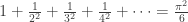$1 + \frac 1 {2^2} + \frac 1 {3^2} + \frac 1 {4^2} + \dots = \frac{\pi^2}6$ , which was proven by Euler via an entirely different method.

Example 2.3. This is a little astounding. Let $f(x) = e^x$ for $-\pi \le x < \pi$ , and again repeated with a period of 2π. The Fourier coefficients give:

$a_0 = \frac{\sinh\pi}\pi$ .
$a_n = \frac{2\sinh\pi}\pi \frac{(-1)^n}{n^2+1}$ .
$b_n = \frac{2\sinh\pi}\pi \frac{(-1)^{n+1}n}{n^2+1}$ .

So we can write $e^x \sim \frac {\sinh\pi}\pi \left[ 1 + \sum_{n\ge 1} \frac{2(-1)^n}{n^2+1}\cos(nx) + \sum_{n\ge 1}\frac{2n(-1)^{n+1}}{n^2+1}\sin(nx)\right]$ , which holds for all $-\pi < x < \pi$ . In particular, for x = 0, we get the rather mystifying identity:

$1 = \frac{\sinh\pi}\pi \left[ 1 - \frac{2}{1^2+1} + \frac{2}{2^2+1}-\frac{2}{3^2+1}\dots\right],$

which you can verify numerically to some finite precision.

Linear Algebra: Inner Products

Leave a Reply Cancel reply

Recent Posts

Archives

Categories

Meta

Pages

Linear Algebra: Inner Products

Share this:

Like this:

Related

Leave a Reply Cancel reply

Recent Posts

Archives

Categories

Meta

Pages