Mathematics and Such

Combinatorial Game Theory VII

Posted on August 15, 2012 by limsup

Lesson 7

[ Warning: another long post ahead. One of the proofs will also require mathematical induction. ]

In this lesson, we will see how some games can be represented by numbers (which can be integers or fractions). We will also introduce the following game.

Hackenbush

Draw a diagram with Light and daRk edges, which is attached to the ground. E.g.

The two players alternately remove an edge from the diagram. After a move, any component which is disconnected from the ground is eliminated. Furthermore, player Left can only remove Light edges while Right can only remove daRk edges. A player wins if he gets to clear the diagram. Hackenbush can also be played with bLue and Red edges.

Integers

First, consider the following configuration.

It is clear that Left is the winning party. In fact, Left has n free moves available to him while Right doesn’t have any. Hence, it makes sense to label the above game by n. Indeed, we will define the following games as positive integers:

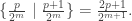
Definition. The game 1 is defined to be {0 | }. And we recursively define the games 2, 3, … as follows:

2 = 1 + 1, 3 = 2 + 1, 4 = 3 + 1, ….

On the other hand, consider the negation of 1, i.e. -1. This is obtained by flipping the colours (Light to daRk and vice versa), so we have the following:

Definition. The game -1 is defined to be { | 0}. And we recursively define the games -2, -3, … as follows:

-2 = (-1) + (-1), -3 = (-2) + (-1), -4 = (-3) + (-1), ….

So the following configuration is equal to –n.

Since -1 is defined to be the negative of 1, we know that 1 + (-1) = 0 by the results in the previous lesson. In other words, when we add and subtract the above games, we are just performing the usual addition and subtraction on integers.

What are the options available for a game which is a positive integer?

From the Hackenbush games above, it is clear that if n is a positive integer, then Left has a single possible move n → n-1 while Right has no available move. Hence, we could also have defined inductively:

1 = {0 | }, 2 = {1 | }, 3 = {2 | }, … , n = {n-1 | }.

Games With Value 1/2

This is our first example of a fraction occurring in a game. Consider the following game G:

Looking at the options of G, we get G = {0 | 1}. It is very tempting to write this as G = 1/2. To check that this is consistent with addition, we need to verify G + G = 1, or equivalently, G + G + (-1) is a second-player win. This is an easy exercise which we’ll leave to the reader.

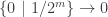
Definition. The game {0 | 1} is denoted by 1/2.

What about -1/2? By definition, it is the negation of 1/2, so it is {-1 | -0} = {-1 | 0}.

Warning : it is not true that 1/2 is the only game G for which G + G = 1 (see exercise 2).

Clearly, 1/2 is a win for Left, so 1/2 > 0. On the other hand, 1/2 + 1/2 = 1, so adding -1/2 on both sides gives us 0 < 1/2 = 1 + (-1/2). Adding 1/2 on both sides again, we get 1/2 < 1. We have, thus, proven:

0 < 1/2 < 1.

Before proceeding to define other fractions, we shall introduce the first method of simplifying games.

Simplification (I)

Consider a general game expressed in this form:

$G = \{A, B, C, \ldots | X, Y, Z, \ldots\}$ .

We claim that if B ≥ A then we can erase A from our list of Left options to obtain $G = \{B, C, \ldots | X, Y, Z, \ldots\}$ . On a heuristic level, this seems obvious since A is a “better” move for Left compared to B. But let’s prove it carefully.

Proof. We write:

$G = \{A, B, C, \ldots | X, Y, Z, \ldots\}$ and $H = \{B, C, \ldots | X, Y, Z, \ldots\}$ .

We need to show that G = H, i.e. G + (-H) is a second-player win. Note that by definition of negation:

$-H = \{-X, -Y, -Z, \ldots | -B, -C, \ldots\}$ .

Now, the second player has an easy strategy as follows: whatever the first player does, he does the reverse in the other component. The only problem occurs if Left starts by taking G → A. Although Right has no corresponding move –H → –A, he can do even better: take –H → -B. The resulting game is now:

$A - B \le 0.$

Recall from last lesson’s exercise that in such a game, if Left starts, then Right wins. But now it’s precisely Left‘s turn, so Right gets to win. Conclusion: G – H is a second-player win, which completes the proof. ♦

Note that the above simplification rule has a twin brother: If X and Y are Right‘s options in the game G, and X ≥ Y, then we can erase X from the list of Right options and the game is still equal to G.

More Fractions

The next step is to look at the game:

Writing the options of G, we get G = {0 | 1/2, 1}. By the simplification rule we just covered, we can remove 1, so G = {0 | 1/2}. A bit of work should convince you that G + G + (-1/2) = 0 (i.e. is a second-player win). So let’s define 1/4 = {0 | 1/2}.

More generally, let’s consider the following game:

$hacken_frac$

We would like to label $G_n = 1/2^n$ . To do that, we need to show that $G_n + G_n = G_{n-1}$ for n = 1, 2, 3… . The proof will be carried out by induction.

Proof. Suppose we already know that $G_n + G_n = G_{n-1}$ for n = 1, 2, … t-1. Then for n = t, we have:

$G_t = \{0\ | \ G_0, G_1, G_2, \dots, G_{t-1}\}.$

It is easy to see that $G_0 > G_1 > G_2 > \ldots$ (it’s not that hard, so we’re leaving it as an exercise) so the game simplfies to $G_t = \{ 0\ |\ G_{t-1}\}$ . Hence it remains to show that:

$\{0\ |\ G_{t-1}\} + \{0\ |\ G_{t-1}\} + (-G_{t-1}) = 0.$

Note that $-G_{t-1} = \{-G_{t-2}\ |\ 0\}$ . To prove that the above game is a second-player win:

Suppose Left starts.
- If Left takes $\{0\ |\ G_{t-1}\} \to 0$ , then Right can take $\{0\ |\ G_{t-1}\} \to G_{t-1}$ , thus leaving the sum 0 and win.
- If Left takes $(-G_{t-1}) \to (-G_{t-2})$ , then Right takes $\{0\ |\ G_{t-1}\} \to G_{t-1}$ . By induction hypothesis, $G_{t-1} - G_{t-2} = -G_{t-2}$ so the game is now $G_t - G_{t-2} < 0$ . Right wins.
Suppose Right starts.
- If Right takes $\{0\ | \ G_{t-1}\} \to G_{t-1}$ , Left takes $\{0 \ |\ G_{t-1}\} \to 0$ , thus leaving 0 and win.
- If Right takes $(-G_{t-1}) \to 0$ , then Left takes $\{0 | G_{t-1}\} \to 0$ also. This gives $\{0\ |\ G_{t-1}\} = G_t$ which is clearly positive. So Left wins.

This completes the proof. ♦

In conclusion, we may label $G_n = 1/2^n$ . Formally, we get the following recursive definition:

1/2 ={0 | 1}, 1/4 = {0 | 1/2}, 1/8 = {0 | 1/4}, 1/16 = {0 | 1/8}, …

More Fractions

Now that we’ve successfully defined fractions of the form 1/2, 1/4, 1/8, 1/16, … , we can now define any rational number of the form $m/2^n$ via addition and subtraction. We call such rational numbers dyadic rational numbers.

Now, one is inclined to naïvely think that we can just take averages: $\{a | b\} = \frac{a+b}2$ . Unfortunately, this is not true in general as the following examples illustrate.

Examples

Consider the game G = {-5 | 2}. If Left starts, he leaves a negative number and Right wins. If Right starts, he leaves a positive number and Left wins. So the 2nd player wins! This means G = 0.
Consider G = {1/4 | 1}. We claim G = 1/2. Indeed, we just need to show G – 1/2 = G + {-1|0} is a 2nd-player win. This is easy (try it!).

Despite this minor setback, we can take averages in some cases.

If p is an integer and m is a non-negative integer, then:

$\{ \frac p {2^m} \ | \ \frac{p+1}{2^m}\} = \frac{2p+1}{2^{m+1}}.$

Proof. First consider the case 2p+1 > 0. Write the RHS (right-hand-side) as a sum of (2p+1) terms, each equal to 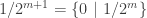$1/2^{m+1} = \{0 \ |\ 1/2^m\}$ . Thus, in this game sum, if Left starts, he has no choice but to play $\{0 \ |\ 1/2^m\} \to 0$ . Likewise, if Right starts, his only move is $\{0\ |\ 1/2^m\} \to 1/2^m$ . By considering these options, we get the game $\{\frac{2p}{2^{m+1}}\ |\ \frac{2p}{2^{m+1}} + \frac 1 {2^m}\}$ which is precisely the LHS. The case where 2p+1 < 0 is similar and is left to the reader.♦

Simplicity Rule

As mentioned earlier, we cannot take averages in a game to simplify it to a number. Due to this subtlety, we need the notion of simplicity:

We introduce an ordering among the set of dyadic rational numbers: the notion of simplicity. This ordering is “partial” in the sense that for some dyadic rational r, s, we are unable to say whether r<s or s>r.

If r has a smaller denominator than s (in reduced fractions), then r is simpler than s.

Among integers, if |a| < |b|, then a is simpler than b.

0 is the simpler than any r.

Examples

-2 is simpler than 3 by criterion 2.
5/2 is simpler than 1/4 by criterion 1.
7/8 and 1/8 cannot be compared; neither is simpler than the other.
4/8 = 1/2 is simpler than 3/8 by criterion 1.

Now we have the following theorem.

Theorem (Simplicity Rule). Suppose G is a game

G = {a, b, c, … | x, y, z, … }

whose options a, b, c, …, x, y, z, … are all numbers. If there is an r such that a<r, b<r, c<r, … and r<x, r<y, r<z, … then G is also a number, and is equal to the simplest dyadic rational r satisfying these inequalities.

As you can tell, this is a highly non-trivial result. The proof will come in three steps:

There exists a simplest dyadic rational r satisfying the inequalities, in the sense that: you cannot find a number s which is simpler than r such that the inequalities hold.
The r found in step 1 satisfies G = r.
Hence such an r must be unique. [ Note that step 1 does not imply that r is unique, since the ordering is only partial. ]

Examples

{-2 | 5} = 0. [ Alternatively : the second player wins so it’s a zero game. ]
{1/2 | 17/4} = 1.
{1/4 | 13/16} = 1/2.
{-1/4 | -1/16} = -1/8.
{17/2 | } = 9.
{-17/2 | } = 0.

Proof of Simplicity Rule

Before start the proof let’s use the following observation.

Let G be a game equal to some dyadic rational number r. Then we can write G as one of the following forms:

{m | n}, where m < n are numbers simpler than r, and m < r < n;

{m | }, where m is a number simpler than r and m < r;

{ | n}, where n is a number simpler than r and r < n;

{ | }.

Why is this true? Well, 0 goes to case (d). If n is a positive integer, then we already know n = {n-1 | } and –n = { | -(n-1)} which are in cases (b) and (c). Finally, any dyadic non-integer can be written as $\frac {2p+1}{2^r}$ for some integer p and positive integer r. But we saw earlier that $G = \frac{2p+1}{2^r} = \{ \frac{p}{2^{r-1}} | \frac{p+1}{2^{r-1}} \}$ .

Now let’s follow the above 3 steps. Recall that:

$G = \{ a, b, c, \ldots | x, y, z, \ldots \}$ ,

where the options a, b, c, …, x, y, z, … are all numbers.

Step 1. This is easy: consider the set of all dyadic rational numbers r satisfying the inequalities a<r, b<r, c<r, … and r<x, r<y, r<z, … . Since the denominator of each r is finite, there must be an element with a smallest denominator (though possibly non-unique). If the smallest denominator is 1 (i.e. r is an integer), break ties by picking the one with the smallest absolute value.

Step 2. We need to show that G + (-r) is a 2nd player win. Suppose Left starts. Since any Left option is less than r, moving in the G-component would result in a negative value (Right wins – bad). On the other hand, suppose he moves in the second component (-r). By the above observation, we may assume the move is (-r) → (-n), where n is simpler than r and r<n. By our choice of r, it follows that either a≥n for some Left option a of G, or n≥x for some Right option x of G.

But n > r > a so the first case is out. We thus have n≥x and Right may win in the resulting game G+(-n) by picking the first component, thus leaving x-n ≤ 0. [ Recall that if a game G satisfies G≤0, then Right wins if Left gets to start first. ] In conclusion, if Left starts in G-r, Right wins.

One can show similarly that if Right starts, Left wins.

Step 3. This follows from the fact that no two distinct numbers are equal, even as games.

In a Nutshell

Here’s a recap of what we’ve learnt.

Impartial games: 0, *1, *2, *3, … .

Numbers: e.g. 1/2, 3/8, 7/16, -5/32, … .

Simplifying a game by removing redundant options.

How to simplify games to numbers using the simplicity rule.

Here’re some further notational simplifications: *1 is usually denoted as just *, while the game G+* is also denoted G*.

Exercises

Jen considers the game G = {1/8 | 1} as well as G – 1/4. She reasons that if Left starts, he could move G → 1/8, leaving 1/8 – 1/4 < 0; and if Right starts, he could move G → 1, leaving 1 – 1/4 > 0. Thus, the 2nd player wins and so G= 1/4. However, this is wrong.
- Use the Simplicity Rule to find the actual value of G.
- Where did Jen’s reasoning go wrong?
Prove that there are infinitely many games G, no two of which are equal, satisfying G + G = 1. Thus, 1/2 is not the only G satisfying this equality.
Prove that for any positive integers n, r, we have $-\frac 1 {2^r} < *n < +\frac 1 {2^r}$ .
Use the simplicity rule to simplify the following games to numbers.
- {-1/2 | 3/8 };
- {-5/2 | -1/2 };
- { 1/2 | 13/16 };
- {5/2 | }.
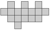
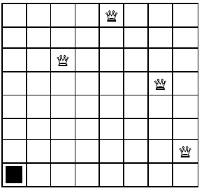
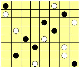
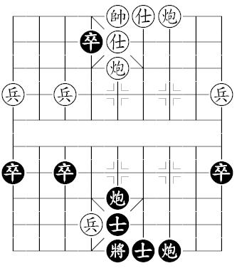
Analyse the following Hackenbush positions and verify their values.

Analyse the following Hackenbush positions and find their values.

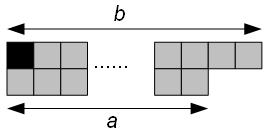
Consider the game of Cutcakes. Given a cake, divided into m × n unit squares, each player at his turn takes a piece of cake and slices it along the edges of the squares, thus dividing the cake into two pieces. In addition, Left can only cut vertically, while Right can only cut horizontally. A typical game may proceed as follows if Left starts. Find the values for m × n Cutcakes, for 1 ≤ m, n ≤ 6.

Each of the following Domineering positions is either a number or a game of the form {m | n}, where m ≥ n are numbers. Compute them.

Posted in Notes | Tagged combinatorial game theory, computer science, game numbers, hackenbush, intermediate, partial games, programming | Leave a comment

Combinatorial Game Theory VI

Posted on August 12, 2012 by limsup

Lesson 6

General Combinatorial Game Theory

[ Warning: the following lesson is significantly longer than the previous ones. ]

Starting from this lesson, we will look at a more rigourous, complete and general theory. Prior to this, in any game configuration both players have the same sets of moves available to them. These are called impartial games. Here, we will look at partial games, whereby a configuration has different options for either player. To distinguish our players, we will call them Left and Right. We will only look at finite games, i.e. we exclude loopy games and games with possible draws. To highlight our theory this week, we’ll introduce the game of Domineering:

Domineering

We have a union of unit squares. E.g.

Each player, at his turn, places a domino (1 × 2 piece) across two neighbouring squares such that no two dominoes may overlap. Left must place his vertically while Right places his horizontally. A player wins if his opponent has no legal move to make. To analyse this game further, let’s have a proper definition of the concept of “game”.

Definition

A game is described as two collections of options, one for Left and one for Right. Each option is in turn a game, so in this way we get a recursive definition of games. This is usually written in the following form:

$G = \{A, B, C, \ldots | X, Y, Z, \ldots \}$

where A, B, C, … are the possible configurations after Left makes a move, and X, Y, Z, … are the possible configurations after Right makes a move. For simplicity, we write 0 for the game { | }, where neither Left nor Right has any move available.

Example

Let’s consider the following Domineering game, with its options:

So the above game is $G = \{G_1, G_2 | G_3, G_4\}$ , where the games $G_1 = \{0 | \ \}$ , $G_2 = \{0 | 0 \}$ , $G_3 = \{\ | 0\}$ and $G_4 = \{\ | \ \} = 0$ . Note that the four games $G_1, G_2, G_3, G_4$ are all different. We can also write the game G in full as follows:

$G = \{ \{ \{ \ |\ \} | \ \}, \{ \{ \ | \ \} | \{ \ | \ \} \}\ |\ \{ \ | \{ \ | \ \} \}, \{\ | \ \} \}.$

But of course no one likes to deal with such unwieldy expressions.

Addition of Games

As before, we can add two games together. Recall the definition of game addition:

The sum of two games G and H is as follows: place G and H side-by-side. At each player’s turn, he must make a move from either G or H, but not both. The move must be legal in the individual game, but there are no constraints on which component to choose from. As before, a player wins if his opponent is left with no legal moves.

Here is an example of addition of two domineering games:

It is clear that addition satisfies:

existence of identity : for any game G, the game 0+G is identical to G;
commutativity : for any games G and H, the games G+H and H+G are identical;
associativity : for any games G, H and K, the games G+(H+K) and (G+H)+K are identical.

These are the common properties one would expect from addition.

Negative of Games

Next, we wish to define the negative of a game G.

Informally, the negative of a game G, written -G, is obtained by exchanging the options of Left and Right recursively. For example, in a game of chess or Chinese chess, the negative of a game is obtained by flipping the board around.

For another example of game negative:

To give a more formal definition of game negative, suppose we write the game as $G = \{A, B, C, \ldots | X, Y, Z, \ldots \}$ . Then the negative is defined recursively via:

$-G = \{ -X, -Y, -Z, \ldots | -A, -B, -C, \ldots\}$ .

Some properties of game negative are intuitively clear:

involution : the negative of the negative of a game is identical to itself;
distributivity over + : the game -(G + H) is identical to (-G) + (-H).

But what about G + (-G) ? Unfortunately, this is clearly not identical to the zero game (it is in fact much more complicated in general). However, we will rectify this apparent anomaly in the up and coming sections. This will be via the concept of game equality.

The Zero Game

We will write the following notation for any game G.

If the second player wins in G, then G = 0. We say G is zero. Note that now, a zero game simply refers to any game where the second player wins, not just the empty game $G = \{\ |\ \}$ .

If Left wins in G regardless of who goes first, then G > 0. We say G is positive.

If Right wins in G regardless of who goes first, then G < 0. We say G is negative.

If the first player wins in G, then G || 0. We say G is fuzzy.

The above cases can be put more succintly in the following table (exercise: fill in the blanks yourself; to see the answer highlight over it):

		Left starts
		Left wins	Right wins
Right starts	Left wins	G > 0	G = 0
Right starts	Right wins	G \|\| 0	G < 0

The definition may appear puzzling at first: why do we regard a game in which the second player wins as a “zero game”? It turns out if G = 0 (i.e. second player win), then the outcome of G + H is the same as that of H for any game H, as can be seen in the following table:

Table 1: Results of Sums of Games

	G = 0	G > 0	G < 0	G \|\| 0
H = 0	G+H = 0	G+H > 0	G+H < 0	G+H \|\| 0
H > 0	G+H > 0	G+H > 0		*
H < 0	G+H < 0		G+H < 0	*
H \|\| 0	G+H \|\| 0	*	*

The table is symmetric about the main diagonal, which is expected since the game sum is commutative (i.e. G+H and H+G are identical games). Instead of proving every entry in the table, we’ll just do it for one entry since the remaining cases are similar.

To show that G>0 and H>0 implies G+H>0 : suppose Left wins in both G and H, regardless of who starts. Now, in the game sum G+H, he simply moves in game G and waits for his opponent for his next move. Whatever his opponent does, Left will simply respond in the same component, as if the other component didn’t exist. This strategy works because, by assumption, he’s guaranteed to have an available move in both G and H.

Note: actually, we can say something about the cases marked *; see exercise 4.

Furthermore, the negative of a game G behaves exactly as we expect it (see exercise 5).

Sum of a Game and Its Negative

Finally, we will explain what’s so nice about this new concept of the zero game:

For any game G, the sum G + (-G) = 0, i.e. G + (-G) is a second-player win.

Why is this so? Look at the two components G and -G and let’s try to figure out a winning strategy for the second player. Suppose the first player makes a move in G – then by definition of –G there is also a corresponding move for the second player in –G. Conversely, whatever the first player chooses to do in –G, the second player can mimic his play in G. In this way, the second player is guaranteed to have a move, so he wins.

[ For a rigourous proof, let’s suppose the first player moves G → A; then the second player counters with -G → -A which is guaranteed to be available by definition of negative. ]

Now we define the game difference of G and H to be

$G - H = G + (-H)$ .

We have just proven that $G + (-G) = 0$ .

Comparison Between Games

Now we extend the above notation to compare any two games G and H. Consider the difference game G – H, which is defined to be the sum G + (-H).

If the second player wins in G-H, then G = H. We say G and H are equal.

If Left wins in G-H, then G > H. We say G is more / larger than H.

If Right wins in G-H, then G < H. We say G is less / smaller than H.

If the first player wins in G-H, then G || H. We say G and H are incomparable.

It’s important to distinguish between “G and H are identical” and “G and H are equal”. The former means that the game options, and all the options’ options, and options’ options’ options etc, are all identical. Thus, if we expand G and H till we’re left with only brackets and “|”, the two strings are identical. On the other hand, if G and H are equal, then it just means G–H is a second-player win, e. g. convince yourself that:

After a few more lessons, you will be able to prove that in general,

Next: given the comparison between G and H, as well as H and K, how does G compare with K? As a precursor, let’s prove that if A=0, then A+B = B. This is quite easy: the difference $(A+B) + (-B) = A+(B+(-B))$ is a sum of two games which are zero. By table 1, the result is also a zero-game.

Now we’re ready to answer our question, for $(G-H) + (H-K)$ is identical to $G + (-H) + H + (-K)$ by commutativity and associativity. We already know that $(-H) + H = 0$ . Adding $G + (-K)$ to both sides, the precursor result tells us that $G + (-H) + H + (-K)$ is equal to $G+(-K) = G-K$ . In summary, table 1 gives us:

Table 2: Comparisons of Games

	G = H	G > H	G < H	G \|\| H
H = K	G = K	G > K	G < K	G \|\| K
H > K	G > K	G > K		*
H < K	G < K		G < K	*
H \|\| K	G \|\| K	*	*

Another important result is the following: if $G = \{A, B, C,\ldots | X, Y, Z,\ldots\}$ then we may replace any option (e.g. A) by another game which is equal (see exercise 6). This shows that we can replace a game G by any equal game G’ whenever it appears.

Application to Impartial Games

We will apply what we’ve learnt so far to rigourously formulate the notions of Nim values. As mentioned earlier, only finite games are considered: no loopy games (i.e. no draws). Let’s define what impartial games are.

A game G is said to be impartial if at every stage of the game, the options available to either player are exactly the same.

Recursively, this means that G is impartial if the set of Left options and the set of Right options are the same, and these options are all impartial.

An alternate definition can be: G is impartial if and only if –G is identical to G. Note that –G can be equal to G without being identical, ergo G can be equal to itself without being impartial.

Examples : all the games we’ve considered in the first four lessons are impartial: namely Nim, Nim-Square, Kayles, Dawson’s Kayles, Grundy’s Game etc.

Since an impartial game G does not distinguish between either player, it follows that either the first player wins, or the second player wins. In other words, G = 0 or G || 0. Notice that in a single Nim heap of n stones, we can remove any number of stones, thus leaving 0, 1, 2, …. or n-1 stones.

So if we wish to consider the special case of a Nim heap of n stones, we should define (recursively):

*0 is the game 0 = { | }.
*1 is the game {0 | 0}.
*2 is the game {0, *1 | 0, *1}.
*3 is the game {0, *1, *2 | 0, *1, *2}.
…
*n is the game {0, *1, … , *(n-1) | 0, *1, … , *(n-1) }.

Theorem. Any Impartial game is equal to *n for some n. Specifically, if G is the game

$\{*r_1, *r_2, \dots, *r_m | *r_1, *r_2, \ldots, *r_m \}$ ,

then G = *n, where $n = mex(r_1, r_2, \ldots, r_m)$ . Recall that the mex of a list of numbers is the smallest non-negative integer which does not occur in the list.

Proof.

We need to show that $G - (*n) = G + (*n)$ is a second-player win. Let’s consider the first player’s options.

If the first player moves $*n \to *m$ for some m < n, then by definition of mex, m occurs among one of the r_i‘s. So the second player counters by moving $G \to *m$ . This gives the game $*m + *m$ , i.e. Nim heaps (m, m) which is a second-player win.
If the first player moves , then we know that by definition of mex.
- If $r_i < n$ , then the second player moves $(*n) \to (*r_i)$ thus giving $(*r_i) + (*r_i)$ which is a second -player win.
- If $r_i > n$ , then the second player moves $(*r_i) \to *n$ , thus giving $(*n) + (*n)$ , which is also a second-player win.

Applying this theorem recursively, we see that any impartial game is equal to a single Nim heap. Next we look at the addition of two Nim heaps.

Theorem. The game sum *m + *n is equal to the game *r, where $r = m\oplus n$ . Recall that the $\oplus$ operation is given by “xor”, or “addition without carry” in binary.

To prove this theorem, we need to show that $(*m) + (*n) - (*r) = (*m) + (*n) + (*r)$ is a second-player win. But this follows from the Nim solution we gave in lesson 2, since by definition there are an even number of ones in every column, when we write r, m and n in binary form.

In short, we have just seen that: (a) any impartial game is equal to a Nim heap, and (b) the sum of two impartial games corresponds to the xor-operation on the corresponding two Nim heaps. This thoroughly justifies our approach used in the first four lessons. Note that it’s possible to skip those lessons and start straight from here, but we wish to provide some interesting examples before burdening you with all these formal definitions.

In a Nutshell

In this lesson, we have learnt that:

the formal definition of games and their negatives;
we can add games and subtract games;
we can compare games: the result can be equality, greater than, less than, or incomparable;
a seemingly complicated game configuration may be equal to a much simpler one;
the ordering and arithmetic operations on games behave consistently with our intuition from real numbers;
an impartial game is equal to a Nim heap *n.

In the next lesson, we will see that some games behave as if they were real numbers. Not only can we have integers, but even fractions. This would greatly simplify computations since we can add and subtract numbers easily.

Exercises

Consider the following diagrams in domineering. Fill in the appropriate symbol between G and 0 in each case, one of = < > or ||.

Prove some of the entries in Table 1.

Now, we extend the comparison notation:

$G \ge 0$ if either G = 0 or G > 0;
$G \le 0$ if either G = 0 or G < 0.

Prove that the notation $G \ge 0$ is equivalent to saying: if Right starts first in the game G, then Left can win. Write down a similar statement for $G \le 0$ . Note: this result will be used repeatedly in subsequent lessons, so do bear them in mind!
Prove that if G || 0 and H > 0, then either G+H || 0, or G+H > 0. Hence, fill in the areas marked * in Table 1. [ Hint: prove that if Left starts in the game sum, he can win. ]
Prove that if G = 0, then –G = 0 as well. Formulate three more statements for the cases G > 0, G < 0 and G || 0.
Prove that if $G = \{A, B, C, \ldots | X, Y, Z, \ldots\}$ is a game and A = A‘, then the game $G = \{A', B, C, \ldots | X, Y, Z, \ldots\}$ obtained by replacing A with A’ is also equal to G.

Posted in Notes | Tagged combinatorial game theory, computer science, domineering, game sum, impartial games, intermediate, nim values, partial games, programming | Leave a comment

Combinatorial Game Theory V

Posted on August 10, 2012 by limsup

Lesson 5

We did mention in the first lesson that CGT covers games without draws. Here, we’ll break this rule and look at loopy games, i.e. games with possible draws. [ To be specific, loopy games are those where it’s possible to move to a state which was previously attained in the game (think of the infinite-check in chess). ]

Let’s start with a specific example.

Square-But-One is a modified version of Square-Game. Start with n > 0 stones. At each player’s turn, he makes one out of two possible moves:
(a) remove a positive square number of stones from the heap; or
(b) if there are a positive even number of stones, he may add one stone.
As before, a player loses if he cannot make a legal move.

Notice that condition (b) gives the possibility of an infinite loop: e.g. convince yourself that 2 will result in a draw. We will still apply our logic from the first lesson:

If n is winning, then there is a move from n to a losing position.
If n is losing, then all possible moves from n lead to a winning position.

Based on this definition, we proceed as before:

0 is clearly losing.
Therefore, 1, 4, 9, 16, … are all winning since they can reach 0.
5 is losing because all possible moves (to 1 or 4) are winning.
Therefore, 6, 9, 14, 21, … $m^2+5$ , …. are winning positions.

Are there any more deductions? It turns out there aren’t – to achieve the next step, we need to find a losing number n, one from which all possible moves lead to winning numbers. It can be proven this is impossible (see exercise 2). So all remaining numbers (numbers not of the form $m^2$ or $m^2+5$ ) are draws!

Nim’s Island

The following is a map of Nim’s Island:

On the island, there is a large swamp surrounding Nim’s house where she stays with her friends, Kim and Tim. Thanks to some stone platforms erected in the swamp, the kids can still freely move about via the above routes. Each platform is large enough to hold any number of people.

Now, two players alternately move one of the three characters along one of the routes. The player who successfully guides all three home, wins the game. Who wins in the above configuration, where the three kids are placed on the gray platforms? Due to the presence of cycles, the game may end in a draw!

Once again, we will label the platforms and house with Nim values, but now we must be extra careful in our analysis! First, the house gets the Nim value of 0.

At each stage, consider an unlabelled (i.e. without Nim value) platform T. Take the set of all platforms accessible from T. Assume that:

the labelled platforms accessible from T have Nim values $*r_1, *r_2, \dots, *r_t$ , and let $r = mex(r_1, r_2, \dots, r_t)$ (recall that the mex of a list is the smallest non-negative integer which does not occur in the list);

every unlabelled platform accessible from T has a path to some other platform which is labelled with *r.

Then we can label the platform T with *r.

Finally, after we’ve labelled all that we can, the remaining platforms are given a Nim value of ∞.

Let’s see how this works in practice. After a while we get these Nim values:

Can we replace the ‘?’ symbol with a Nim value?

There is a labelled platform accessible from it. The Nim value there is given by *2. So we’re inclined to label ‘?’ with mex(2) = 0.
There is an unlabelled platform accessible from it. Furthermore, the unlabelled platform connects to the house (Nim value = 0).

So by definition, we should replace the ‘?’ symbol with 0. After some effort, we get the following:

Winning Positions

It’s a little tricky to interpret the Nim values now, since some of these are infinite (∞)! What should we do with them? Here’s the recipe:

If all Nim values are finite, play as if we’re playing Nim.

If exactly one Nim value is infinite ∞,

if there is a path from this ∞ to a finite Nim value *m, such that *m together with all the other Nim values is a losing position, then the original game is a winning position;

if no such path exists, it’s a draw.

If at least two Nim values are infinite, the game is a draw.

The three positions in our problem give 0, *1, *2, which is a win for the first player. The winning move is given by *2 → *1.

Winning Strategy

Let’s figure out why the above recipe works, by considering various cases.

Take case 1 in the recipe, where all three positions have Nim values. If your opponent shifts one of the Nim values to , what should you do?

Answer: if your opponent shifts *r to ∞, then by definition, there must be a move from this ∞ to a different *r. Make that move. Can your opponent delay his defeat indefinitely by moving to ∞ repeatedly? No, because all the *r labels were obtained after finitely many iterations of the labelling process.

Take case 2(i) in the recipe: suppose two positions are labelled *r and *s but the third one is labelled ∞, such that there is a move from ∞ to $*(r\oplus s)$ . What should you do?

Answer: this case is quite obvious. Make the move $\infty \to *(r\oplus s)$ . The resulting Nim game is a losing position by case 1.

Take case 2(ii) in the recipe: suppose we still have *r, *s and ∞, but now there is no move from ∞ to $*(r\oplus s)$ . What can you do?

Answer: first, you can’t win here. Regardless of what you do, you’ll end up with case 2(i) , case 2(ii), or case 1 with a non-zero Nim sum – all of which are either draws or winning positions for your opponent!

So the best you can hope for is a draw, which you can attain by adopting the following.

Consider all possible Nim values reachable from ∞. If one of these values is not *t’, where $t' < t := r \oplus s$ , then just move the Nim part (*r, *s) to *t’. You’re still in case 2(ii) so you’re safe.

If not, then the Nim values 0, *1, *2, … , *(t-1) are all reachable from ∞. By assumption, *t is not reachable from ∞. Now why is the position ∞ and not *t? It follows that there is a move from ∞ to another place c (also labelled ∞) such that there is no move from c to *t. The resulting position is then in case 2(ii).

Take case 3 in the recipe: suppose we have two or more ∞. What can we do?

Answer: not much, since cases 2(i) and 2(ii) are either draw or first-player win. Your safest bet is to loiter around case 3 by moving from ∞ to another ∞. Ok, maybe you can move to case 2(ii), but why take the risk?

Exercises

Consider a modification of Square-But-One: begin with n > 0 stones as before. Each player, at his turn, either (a) removes a square number of stones, or (b) add a stone if the number of stones is odd. Analyse this game for n < 40: which numbers are winning numbers, which are losing numbers, and which result in a draw?
(Hard) Prove the assertion that in Square-But-One, any number not of the form or ends in a draw. One possible approach:
- Prove that if n > 5, then n-1 and n-4 cannot both be squares.
- Prove that if n > 10, we cannot have $n-1 = a^2$ and $n-4 = b^2+5$ for some integers a, b.
- Using (a), (b) and two more such results, prove that any number not of the form $m^2$ or $m^2+5$ ends in a draw.
Take the game of Snakes-and-Adders. Start with some counters scattered on the board (e.g. as below). Two players alternately make a move, by advancing a counter at least 1 step, and at most 4 steps ahead. There’re no constraints on which counter to pick from and the number of steps to move, as long as it does not go beyond “HOME”. When a counter reaches the tail of an arrow, it must follow it to its head (like snakes-and-ladders). The player who moves all the counters HOME wins. Each square can hold any number of counters. Analyse the board and label each square with its Nim value (either *r or ∞).

The game “Fair Shares and Varied Pairs” is played as follows: start with 6 almonds and arrange them in some heaps. Two players alternately make one of two possible moves, either (a) divide any heap into two or more equal-sized heaps, or (b) merge two heaps of different sizes to form a single heap. A player wins when his opponent cannot make a legal move, i.e. when he leaves (1, 1, 1, 1, 1, 1) for his opponent. Analyse the game and find all winning positions, losing positions and draw positions – no need to compute the Nim values. Note: there are altogether 11 positions.
If you know programming, analyse “Fair Shares and Varied Pairs” for 1-15 almonds. Can you formulate a general result?
In Epstein’s Put-or-Take-a-Square, we’re given a heap of n stones (n > 0). Let $m^2$ be the largest square number which does not exceed n. Now, the next player may choose to either add or subtract $m^2$ stones to the heap. E.g. with 7 stones, you’re allowed to put or take 4 stones. Explore this game for heaps of remoteness 3 or below. [ Note : the case of n = 92 is interesting because it has remoteness 11. ]
(Hard) A horsefly moves on a board extended downwards infinitely (see diagram below). At each move, a player picks up a horsefly and makes one out of at most six possible moves. Furthermore, a horsefly may not reverse its previous move. Now the objective of this game is slightly different from previous games: the first player to move any horsefly home wins the game. As before, a square can hold any number of horseflies. What is a good move for the first player in the starting position below? [ Note: my earlier homepage had a detailed – and excruciatingly wordy – analysis of this game. ]

Posted in Notes | Tagged basic, combinatorial game theory, computer science, impartial games, loopy games, nim values, programming | 5 Comments

Combinatorial Game Theory Quiz 1

Posted on August 8, 2012 by limsup

This quiz lasts 70 minutes and covers materials from lessons 1-4.

For A-C, determine whether the following Nim games are first or second-player wins. There is no need to find the winning move. (10 points)
1. (10, 15, 17, 19)
2. (7, 14, 17, 24)
3. (19, 18, 5, 11)
4. If (5, 7, 9, m) is a second-player win, what is m?
The following Nim games are all first-player wins. Find ALL possible winning moves from each game. (10 points)
1. (5, 8, 10, 13, 17)
2. (5, 14, 15)
3. (11, 12, 13, 15)
In the game Cube Game, start with several heaps of stones. Two players alternately remove a positive cube number of stones from exactly one of the heaps, and the player who removes the last stone wins. Find the Nim value of one heap of n stones, for n between 45 and 50 inclusive. (12 points)

0	1	2	3	4	5	6	7	8	9	10	11	12	13	14	15	16
0	*1	0	*1	0	*1	0	*1	*2	0	*1	0	*1	0	*1	0	*1

17	18	19	20	21	22	23	24	25	26	27	28	29	30	31	32	33
*2	0	*1	0	*1	0	*1	0	*1	*2	*3	*2	*3	*2	*3	*2	*3

34	35	36	37	38	39	40	41	42	43	44	45	46	47	48	49	50
0	*1	*3	0	*1	0	*1	0	*1	0	*1

Determine whether the following are first- or second-player wins. (7 points)
- (21, 28, 33)
- (44, 49, 50)
- (33, 37, 40, 45)

Find ALL possible winning moves from the following Cube Game configurations. (16 points)
- (6, 7, 8)
- (24, 25, 26)
- (34, 35, 36)
In a certain game, moves a, b, c, d, e and f result in remoteness values of 5, 7, 8, 9, 10, 11 respectively. What is the best move for the first player? What is his worst move? Explain your answer briefly. (6 points)
Suppose the remoteness values were 4, 8, 10, 12, 20, 22 instead. Same as above: what are the best and worst moves for the first player? (6 points)
Consider the game of Triple Kayles: given a continuous row of n bottles, a valid move knocks down three neighbouring bottles, possibly separating the row into two rows.

A player loses if there’s no valid move for him (i.e. when each row has only 1 or 2 bottles, the next player loses). Find the Nim values of Triple Kayles for one row of n bottles, for 15 ≤ n ≤ 20. Also, prove that if the Nim value for n is *0, then either n=1 or n is even. (14 points)

0	1	2	3	4	5	6	7	8	9	10	11	12	13	14	15	16	17	18	19	20
0	0	0	*1	*1	*1	*2	*2	0	*3	*3	*1	*1	*1	0

Remember Wythoff’s Queens? Each queen can move in three possible directions:

Now consider the chessboard below: at each player’s turn, he picks just one queen and moves an arbitrary number of moves either left, down or diagonally left-down. Each square can hold any number of queens at any time.

But the rules have changed now: the first player to put any queen onto the black square wins. Analyse the above board: who wins? (14 points).

Some Notes

When I conducted the course in 2008, the average score was 73.5 out of 95 with a standard deviation of 8.3. Yup, the students were pretty good! Either that, or the quiz was too simple. 😛
The students ranged from years 1-4 (equivalently, Sec. 1-4 or grades 7-10).
Q7 was pretty tricky, and if my memory serves me well, only 2 out of 20+ students solved it correctly.
Some students were tricked by Q4 because <rot13>gurl qvq abg ernyvfr gung avz inyhrf, hayvxr gur avz urncf, pna npghnyyl vapernfr</rot13>!

Posted in Homework | Tagged basic, combinatorial game theory, computer science, impartial games, nim, nim values | Leave a comment

Combinatorial Game Theory IV

Posted on August 6, 2012 by limsup

Lesson 4

In this lesson, we will work on a large class of games, known as take-and-break games. First consider a simple example.

Kayles

Kayles is an example of a take-and-break game:

Start with a few heaps of contiguous bottles, e.g.

Each player alternately knocks down one or two adjacent bottles, until there is nothing left. The player who removes the last bottle wins. Note that knocking down a bottle or two splits a heap into two smaller heaps unless the bottle(s) are at the end of the heap.

An example of a valid move of the above game is:

which divides the middle heap into two. This can then be followed by:

etc. We will analyse this game using the theory we’ve just developed. First consider the Kayles game with one single heap of n bottles. If we can find the Nim value of one heap, then we can certainly find the solution to any number of heaps.

Sum of Two Games

First we define the sum of two games G+H to be the combined game, whereby at each turn, a player can choose a valid move in G or a valid move in H but not both – there are no constraints on which component (G or H) he can choose. The player who is unable to make a valid move in either G or H loses in this combined game G+H.

For example, consider the sum of Chinese chess and international chess, as below. (In this particular game sum, though, it’s not clear how to determine the winner.)

For another example of game sum, consider the two Nim games (3, 4, 5) and (7, 10, 11). Their sum is the Nim game (3, 4, 5, 7, 10, 11). More generally, any Nim game can be broken up as the sum of its individual heaps, i.e. (3, 4, 5) is the sum of the three Nim games (3), (4) and (5). The Nim-Square game in the previous lesson is then merely a sum of one or more copies of the Square-Game.

Having described the concept of sum, we may state the main result.

If G has Nim value *m and H has Nim value *n, then the sum G+H has Nim value $*(m \oplus n)$ , where $\oplus$ is the “addition without carry” operation defined in the last lecture.

We will not prove this theorem here, but eventually we will when we introduce the general abstract theory. For now let us contend ourselves with some heuristic understanding.

The idea is that if G has Nim value *m, then we saw in the previous lesson that one can replace the game G by *m in a game sum without significantly altering the game play. Oh there’re some slight differences alright, such as the ability for the players to increase the Nim value. However, this makes no difference to the winning player, since he can make a winning move to a position with a smaller Nim value. It makes no difference to the losing player either, since his opponent can push back the Nim value to the old one.

Confused? Hopefully, the following example gives you a better idea.

Solving Kayles

Let $K_n$ be the game of Kayles with a single heap of n bottles. Our objective here is to compute the Nim value of $K_n$ . It is easy to see that K₀, K₁ and K₂ have Nim values 0, *1, *2 respectively. What about $K_n$ for higher values of n?

Let’s suppose the following Nim values are known:

n	0	1	2	3	4	5	6	7
K_n	0	*1	*2	*3	*1	*4	*3	??

To compute the Nim value of K₇, we need to consider all possible positions after one move: K₆, K₁+K₅, K₂+K₄, K₃+K₃, K₅, K₁+K₄, K₂+K₃. These have the following Nim values:

$K_6 : *3$ ;
$K_1 + K_5 : (*1) + (*4) = *(1 \oplus 4) = *5$ ;
$K_2 + K_4 : (*2) + (*1) = *(2 \oplus 1) = *3$ ;
$K_3 + K_3 : (*3) + (*3) = *(3 \oplus 3) = 0$ ;
$K_5 : *4$ ;
$K_1 + K_4 : (*1) + (*1) = *(1 \oplus 1) = 0$ ;
$K_2 + K_3 : (*2) + (*3) = *(2 \oplus 3) = 1$ .

The Nim value of K₇ is the smallest Nim value which does not occur among all its moves, i.e. *2 in this case.

Playing Kayles

In our definition of Kayles, we used the example of a game with heaps of (3, 4, 5, 2, 5). Let’s analyze this game. The Nim values of the heaps are *3, *1, *4, *2, *4, with a combined Nim sum of 0. So the second player wins.

Suppose the first player makes a move 4 → (2, 1). How would you respond? Well, since the resulting game (3, 2, 1, 5, 2, 5) has Nim values *3, *2, *1, *4, *2, *4 with a Nim sum of *2, one possible move is *3 → *1, which corresponds to 3 → 1.

Exercises

Dawson’s Kayles has the same rules as Kayles, except that every player must remove exactly two contiguous bottles. Consider the following configurations which describe the number of bottles in each heap. Are the following first- or second-player wins?
- (12, 13, 14);
- (8, 9, 10, 13).
If you know programming, find the Nim values for Dawson’s Kayles and Kayles up to n=150. Do you see a pattern?
In Grundy’s Game, we begin with some heaps of stones. Here, the only legal move for each player is to split a heap into two smaller heaps of differentsizes. Solve this game for:
- (10, 11, 12);
- (13, 14, 15).
In Lasker’s Nim, we have one or more heaps of stones. Each player, at his turn, takes a number of stones from any one heap, and may in addition splits that heap into two smaller heaps. Analyse Lasker’s Nim for three heaps, of sizes 7, 11, 15. How does Lasker’s Nim differ from ordinary Nim?
Analyse two-dimensional Kayles: start with an m × n board. At each player’s turn, he picks a board and removes a horizontal or vertical slice of width 1, possibly breaking the board into two smaller boards. The slice must be along the edge of the grid squares. For example, a game on a 7 × 4 board may proceed as follows:

In Treblecross, also known as one-dimensional tic-tac-toe, you start with an n × 1 board, where initially all n squares are empty. Two players alternately pick an empty square and fill it with an ‘X’. The first player to fill in three X’s in a row wins. Analyse the n× 1 board for n up to 15: i.e. determine who wins.For 11 ≤ n ≤ 15, if the first player wins, find the winning move.

(For chess players) In Dawson’s Chess, two players start with an n × 3 chessboard, with pawns of different colours lining opposite edges. At each player’s turn, he may move his own pawn or capture an opponent’s pawn, where the rules for movement and capturing are the same as that of chess. Furthermore, capturing is obligatory, i.e. if a player has a chance to capture his opponent’s pawn, he must do so; if more than one capture is available, he can choose any one of them. Analyse the following board.

Posted in Notes | Tagged basic, combinatorial game theory, computer science, impartial games, nim values | 1 Comment

Combinatorial Game Theory III

Posted on August 5, 2012 by limsup

Lesson 3

We’ve learnt Nim and we’ve learnt the Square Game. Now, let’s combine them and consider the following game, which we shall name Nim Square.

Start with r heaps of stones, of sizes $n_1, n_2, \dots, n_r > 0$ . Play alternates between two players: at each player’s turn, he must pick a heap and remove $m^2$ stones from it, where m is a positive integer. As before, he can remove stones from one and only one heap.

Here is an example of a play between two players for (1, 2, 9):

$(1,\mathbf{2},9) \to (1,\mathbf{1},9) \Rightarrow (1,0,\mathbf{9}) \to (1,0,\mathbf{5}) \Rightarrow (1,0,\mathbf{1}) \to (\mathbf{1},0,0) \Rightarrow (0,0,0).$

Thus the second player wins again. It turns out there is a very neat method of solving Square Nim, which is generalisable to a vast class of games called impartial games. A more exact definition of this term will be given in future lessons.

Nim Value

Let us return to the original Square Game, which can be played on any number n. Now, to each n we assign a value *m to it, where m is a non-negative integer. Called the Nim value of n, it is recursively defined as follows:

The number 0 has Nim value *0 (also written *0 = 0).

For each n, we look at all possible moves from n, and label the results $m_1, m_2, \dots$ . Suppose these numbers have Nim values $*r_1, *r_2, \dots$ respectively, then the Nim value of n is defined to be *r, where r is the smallest non-negative integer which does not occur among $r_1, r_2, \dots$ .

For convenience, we will write $r = mex(r_1, r_2, \dots)$ . E.g. mex(0, 1, 2, 6, 2, 10) = 3 since 3 is the smallest non-negative integer which does not occur in the list. Also, note that mex( ) = 0.

As a demonstration, suppose we have the Nim values for n=0, … 13:

0	1	2	3	4	5	6	7	8	9	10	11	12	13	14
0	*1	0	*1	*2	0	*1	0	*1	*2	0	*1	0	*1	?

Let us compute the Nim value of 14: now 14 has moves to 13, 10, 5, which have Nim values of *1, 0, 0 respectively. Hence the Nim value of 14 is *2. Check that the Nim value of 15 is 0.

Now we are ready to describe our strategy for Nim Square (after which, the explanation will follow). Let’s consider the above configuration (1, 2, 9).

Replace every number by its corresponding Nim value: i.e. (*1, 0, *2).

Now imagine yourself playing this Nim game. What would be the appropriate response in this game? In our case it’s got to be *2 → *1.

Find the corresponding move in the Nim Square game. Here, *2 → *1 translates to 9 → 8. In general, there may be more than one possibility.

Thus, a correct response for the first player is (1, 2, 9) → (1, 2, 8).

Why Does It Work?

It’s natural to inquire how it works. Here’s a brief sketch:

Suppose it’s the winning player’s turn. He figures out the correct Nim move: *r → *s where s < r and *r refers to the Nim value of the number n. Why can he find a corresponding move in n? Because, by definition of the Nim value, any number s < r must appear as a Nim value for one of the moves n → m, since r is the smallest value which does not occur as a Nim value of its moves.
Suppose it’s the losing player’s turn. He makes a move corresponding to the Nim move *r → *s, where s ≠ r by definition of r. If s < r, then this move indeed does correspond to a move in the Nim game. But what if s > r? Then since the current number now has Nim value *s with s > r, there’s definitely a move from this number to another with Nim value *r. In short, it does not matter if the Nim value increases, we just bring it back down.

Example

Let’s look at our example of (1, 2, 9) again, and see how the game proceeds. Take note of the interplay between the original game and the corresponding Nim game.

First player		Second player
Nim Square	Nim	Nim Square	Nim
(1,2,9) → (1,2,8)	(1,0,2) → (1,0,1)	(1,2,8) → (1,2,4)	(1,0,1) → (1,0,2)
(1,2,4) → (1,2,3)	(1,0,2) → (1,0,1)	(1,2,3) → (1,1,3)	(1,0,1) → (1,1,*1)
(1,1,3) → (1,1,2)	(1,1,1) → (1,*1,0)	(1,1,2) → (1,0,2)	(1,1,0) → (*1,0,0)

As stated earlier, the winning player (in this case, the first player) always imagines himself to be playing the corresponding Nim game, then translates the Nim move to a move in the original game. Notice that unlike the case of Nim, the nim values here may actually bob up and down. If the losing second player attempts to raise the nim value and confuse the enemy, the first player calmly restores it back to the original nim value.

Exercises

Calculate the Nim values for Wythoff’s game for the positions (m, n), where $0 \le m, n \le 8$ .
Consider the game Wythoff’s Queens (also known as Wyt’s Queens). Each queen is allowed to move, in three possible directions, an arbitrary number of squares.

Now consider the chessboard below: at each player’s turn, he picks just one queen and moves an arbitrary number of moves either left, down or diagonally left-down. Each square is allowed to hold any number of queens at any time. The winner of the game is the one who puts all the queens on the lower-left square. Who wins in the board below?

Unlike a queen, a rook can only move downwards or left. Replace the queens in Wythoff’s Queens with rooks instead. Solve the resulting game Wythoff’s Rooks.
Compute the Nim values of the following:
- Square Game for n = 0, …, 20.
- Cube Game for n = 0, …, 20: the Cube Game is exactly the same as the Square Game, except that at each turn, a player must subtract a perfect cube instead of perfect square. E.g. 15 → 7 is a valid move since 8 is a perfect cube.
The game of White Knights is played on chessboard with a (surprise, surprise!) white knight situated on a square. Unlike a real chess knight, our knight here has only four valid moves (see diagram below). Furthermore, though he started off with some luggage, he has the uncanny habit of losing his belongings over time. Now, two players alternately move by doing (A) or (B), but not both:
1. Take away an arbitrary number of pieces of luggage.
2. Make a move of the knight.
Whoever makes the knight rest on one of the four home squares with no belongings, wins the game. Starting with the configuration below, who wins? If the first player wins, describe a winning move.

Consider the Nim-Square-Cube combination: start with three heaps of stones, of sizes (a, b, c) respectively. Two players alternately make a move by performing one of the three possible actions:
- removing any number of stones from the first heap; or
- removing a positive square number of stones from the second heap; or
- removing a positive cube number of stones from the third heap.
An example of a game play might be:

$(7,9,9) \to (7,5,9) \Rightarrow (7,4,9) \to (7,4,1) \Rightarrow (5,4,1) \to (5,0,1) \Rightarrow \dots$

In each of the following games, who wins – the first or second player? If the first player wins, find a good move for him.
- (3, 11, 17);
- (9, 14, 19).
The game of Binary Nim is played as follows: start with three heaps of stones of sizes (100000, 100001, 100002). At each player’s turn, he takes away a number of stones from one and only one heap, where the number is a power of two ( $2^r$ , for some non-negative integer r). Who wins in this game?

Posted in Notes | Tagged basic, combinatorial game theory, computer science, impartial games, nim values, programming | Leave a comment

Combinatorial Game Theory II

Posted on August 4, 2012 by limsup

Lesson 2

In this lesson, we will focus on a special type of game called Nim. Although it’s only one out of infinitely many possible games, understanding it in depth will be very beneficial in analysing a much larger class of games, known as impartial games. (The exact definition of this term is deferred until a later lesson.)

The rules of this game are as follows:

Start with r heaps of stones, of sizes $n_1, n_2, \dots, n_r > 0$ . Play alternates between two players: at each player’s turn, he must pick a heap and remove as many stones as he wants from it, possibly even emptying the heap. However, he can remove stones from one and only one heap.

Here is an example of a game between two players:

$(3,5,\mathbf{8}) \to (3,\mathbf{5},1)\Rightarrow (\mathbf{3},2,1) \to (0,\mathbf{2},1) \Rightarrow (0,\mathbf{1},1) \to (0,0,\mathbf{1})\Rightarrow (0,0,0).$

Thus the second player wins in this match.

Of course, we could do our analysis as in the previous lesson: to check whether (3, 5, 8) is winning or losing, we could iteratively compute the status of $(a, b, c)$ for $0 \le a \le 3, 0 \le b \le 5, 0 \le c \le 8$ . But this would require us to compute the status for 3 × 5 × 8 = 120 positions, even for a simple configuration like (3, 5, 8), which is way too much work. Thankfully, there is a beautiful solution for the problem.

Binary Representation

If you understand what binary representation is, you may skip this section entirely. The crux of the matter is the following result:

Every positive integer is uniquely representable as a sum of distinct powers of two (i.e. 1, 2, 4, 8, 16 … ).

The keyword here is “distinct”. To write a number n as a sum of distinct powers of 2, let $m=2^r$ be the largest power of 2 which does not exceed n. Now consider the difference $d = n - 2^r$ . If d = 0, then $n=2^r$ and there is nothing left to do. Otherwise, d > 0. We claim that $d < 2^r$ ; indeed, if $d \ge 2^r$ then $n = d+2^r$ would be at least $2^r + 2^r = 2^{r+1}$ which contradicts the maximality of r. (q.e.d.)

Example : let’s take n=25. To take the largest power of two which is at most 25, we have to pick $2^4=16$ . The difference is:

$25 - 2^4 = 9$ .

Now do the same with 9: the largest power of two not exceeding it is $2^3 = 8$ and the difference is:

$9 - 2^3 = 1$ .

Finally $1 = 2^0$ so we can write $25 = 2^4 + 2^3 + 2^0$ . We will write this more compactly as follows:

$25 = (11001)_2$ .

This is known as the binary representation of 25. We can add as many leading zeros as we want:

$25 = (11001)_2 = (011001)_2 = (0011001)_2 = \ldots$

which is akin to 37 = 037 = 0037 = … in decimal representation.

Solving Nim

Now we are ready to describe our strategy for playing Nim perfectly. For simplicity, we consider only three heaps of stones: (a, b, c), where a, b, c > 0, and take the example a = 17, b = 25, c = 13. First, write a, b, c in binary notation and align them on the right. E.g.

17 = (10001) = 16 +           1
25 = (11001) = 16 + 8 +       1
13 = (01101) =      8 + 4 +   1

Now count the number of ones in each column and note their parities. In our example, we have (from left to right): 2, 2, 1, 0, 3. Their parities are even, even, odd, even, odd respectively. The big theorem is as follows:

The above Nim configuration is a losing position if and only if there is an even number of ones in each column.

Hence, the above configuration is winning (i.e. first player wins) since there are an odd number of ones in the rightmost column. One naturally asks for a proof to this theorem. Instead of a rigourous proof, we will instead explain a winning strategy, from which the proof should be apparent. For now, let’s look at another example.

Example

Consider the Nim game (30, 15, 27, 10). To compute its status, let us write:

30 = (11110) = 16 + 8 + 4 + 2
15 = (01111) =      8 + 4 + 2 + 1
27 = (11011) = 16 + 8 +     2 + 1
10 = (01010) =      8 +     2

Now there are an even number of ones in every column, so the second player wins.

Playing Nim

Knowing the status of the game position is just half the battle won – you need to know how to exploit a winning position to obtain an eventual victory. Below, we will explain how to do this, by looking at the case of (17, 25, 13) above. As before, write:

17 = (10001)
25 = (11001)
13 = (01101)

Starting from the leftmost position, find the first column c which has an odd number of ones:

17 = (10 [0] 01)
25 = (11 [0] 01)
13 = (01 [1] 01)

Next, pick a heap number m which has a one in that column. Such a heap must exist, since otherwise, there’d be no 1’s in that column (and thus, an even number of ones). In our example, we must take m = 13. Now remove the binary digits of m from column c to the right.

17 = (10 001)
25 = (11 001)
 ? = (01 ***)

Fill in our desired binary digits in order to have an even number of ones in each column:

17 = (10 001)
25 = (11 001)
 ? = (01 000)

Note that this is a losing position by our theorem, so it would do us good to leave this configuration for our opponent. Also, such a move is always possible since we’re flipping the ‘1’ in column c to ‘0’, and no bits to the left of c are changed. So the resulting number is always smaller than m. Since (1000) = 8 in binary, in our example, a good move would be:

(17, 25, 13) → (17, 25, 8).

Thus, we see that given a winning position, it is always possible to move to a losing position for the opponent. That’s only half the theory; we also need to explain why every move from a losing position results in a winning one.

The XOR Operation

Given a Nim game $G = (n_1, n_2, \dots, n_r)$ if $n_1, n_2, \dots, n_{r-1}$ are fixed, then there’s only one possible $n_r$ for which G is a losing position. Indeed, suppose r= 3 and $n_1 = 37, n_2 = 52$ . Then to compute $n_3$ , we write the binary representations:

n1 = 37 = (100101)
n2 = 52 = (110100)
n3 = ?? = (******)

For each column of $n_3$ , there’s a unique bit such that the total number of ones in that column is even:

n1 = 37 = (100101)
n2 = 52 = (110100)
n3 = ?? = (010001)

This shows that $n_3 = 17$ is unique and also gives us a recipe for calculating it: simply add the two numbers in binary and ignore any carry which might occur. Addition has never been easier! Just perform 0+0 = 0, 0+1 = 1+0 = 1, 1+1 = 0 and forget the carry. This operation is called XOR for exclusive-or, or sometimes just addition without carry and denoted by $n_3 = n_1 \oplus n_2$ .

Incidentally, this also explains why every losing position must lead to a winning one in the next move. For if $(n_1, n_2, \dots, n_r)$ were a losing position, then:

$n_1 \oplus n_2 \oplus \dots \oplus n_r = 0$ .

Another way of writing this would be $n_r = n_1 \oplus n_2 \oplus \dots \oplus n_{r-1}$ . Hence, if the first player makes a move from $n_r$ , then it would result in $n_r' \ne n_1 \oplus n_2 \oplus \dots \oplus n_{r-1}$ which is a winning position. Since there’s nothing special about the last heap $n_r$ , any move would also result in a winning position.

Exercises

Determine the status of the following Nim games:
- (17, 18, 13),
- (18, 14, 9, 21).
For the games in Q1 where the first player wins, find a good move for him.
Given that the Nim game (15, 20, 7, m) is a second-player win, what is m?
Mum has baked a large almond cake which is divided into unit squares as below:

Unfortunately, the black square is burnt and inedible. Now Alice and Bob play a game as follows: each child alternately cuts the cake into two (possibly unequal) pieces, by a horizontal / vertical cut which is along a gridline. He/she then eats the edible piece and leaves the other behind. Whoever is left with the burnt piece is deemed to have lost and must do the dishes. If Alice starts the game, can she avoid the dishes?

In Northcott’s Game, each player controls counters of a certain colour (either black or white). At his turn, he may arbitrarily shift his counters left or right any number of squares. However, no counter may jump over another counter. The player who’s unable to make any move loses. If black starts first, who wins, or will the game never end?

In Misere Nim, the rules are exactly the same as Nim with one caveat: the person who takes the last stick loses the game instead of winning. Based on your understanding of classical Nim, find a strategy for Misere Nim. Explain how the strategies for the two games differ.
(Hard) In Nimble, we have coins in the following strip: each square contains at most one coin. Play alternates between two players. Each player, at his turn, picks up any coin and shifts it to some position on its left – without sliding off the strip and without jumping over another coin. Does the first or second player win in the following configuration?

Analyse the following Chinese Chess position : who wins?

This interesting mathematical game is the subject of some research recently. The game of Chomp is played as follows: start with an m-by-n grid of squares. Two players take turns cutting out a piece of the board by (i) picking any unit square on the board, and (ii) cutting away all squares to its right and below. Whoever is forced to take the top-left square loses.

Find a winning strategy for the first or second player on an n-by-n square board.
Find a winning strategy for the first or second player on an 2-by-n square board.
Determine whether the first player wins in the following configuration. (P. S. The answer depends on a and b.)

(Hard) Prove that, in general, the first player wins on any m-by-n grid if mn > 1.

Posted in Notes | Tagged basic, combinatorial game theory, computer science, impartial games, nim, programming | Leave a comment

Combinatorial Game Theory I

Posted on August 2, 2012 by limsup

[ Prerequisites required: none for now. ]

In the middle of 2000, I was waiting to go to graduate school and had a bit of free time on my hands. So I decided to prepare a website which teaches combinatorial game theory (CGT) methodically. The subject fascinated me in various ways: it was simple enough that a sufficiently motivated primary school child can probably learn much of it. Yet at the same time, notes and books on it were scarce. Recall that back then, there was no wikipedia, youtube, online courses, and even lecture notes were quite scarce on the internet. Due to time constraints and possibly waning interest, the notes were never complete.

Fast forward another 8 years, and I decided to give it another shot. This time, I offered to teach the course as an elective at NUS High School. It was a stressful yet tremendously rewarding experience since I believe there’s no precendent for teaching CGT to pre-university (grades 7-12) students. The challenge was in dividing the materials into discrete packages, so that there’s something interesting for the students to learn every week. I must say I was reasonably pleased with the results, though no doubt there’s much room for improvement.

Since I don’t think I’ll be conducting the course again, here’re the notes. Hopefully, they’re fit for public consumption. There should be 12-13 lessons in all. Stay tuned! 🙂

[ My first website (together with all personal homepages on the server) got taken down recently. However, they’re still available at archive.org if anyone’s interested. ]

Lesson 1

Combinatorial game theory (CGT) explores games with the following properties:

Deterministic: no luck is involved.
Finite: the game is guaranteed to end within a finite time.
Two-player: only two players are involved.
No draws: there must be a winner.
Open: all information and legal moves are known to both players.
The player who is unable to make a move loses.

Note that many classical games do not fall under this criteria. Even so, the theory is of interest for a variety of reasons.

Many interesting games do fall under this criteria.
Researchers in A.I. (artificial intelligence) find it useful in game programming.
The theory offers some very deep insight into classical games. E.g.
- Dots-and-Boxes
- Go (Weiqi) endgames

The case for Weiqi is especially interesting, since it has been known to solve Weiqi endgame problems which are tricky enough to stump 9-dan professionals(!). Unfortunately, we won’t delve into this aspect as it is rather difficult.

Course Requirements

This course does not assume prior knowledge of other areas of mathematics. However, some familiarity with classical games like Chess and Chinese Chess may come in handy for certain problems. Also, although homework submissions are mostly proof-free, the course lectures will involve quite a few proofs, especially towards the later part.

No programming is required, but it’s definitely fun to program the games covered in the course to see the outcome for yourself. Challenge your friends and stump them!

Square Game

Consider the following game, which we shall call the Square Game (for lack of a better name):

Start with a positive number of stones and play alternates between players A and B. At each player’s turn, he must remove m stones, where m is a positive square number. The player who is unable to make a move loses. Equivalently, the player who removes the last stone wins.

Here’s an example of how the game may proceed:

$23 \to 22 \Rightarrow 18 \to 14 \Rightarrow 10 \to 9 \Rightarrow 0$ ,

So the second player wins the game by removing all stones. The nagging question is: could the first player have won by making some better move? Indeed, we shall soon see that the first player’s second move (18→14) was a very bad one. He could have won by taking (18→17) instead.

To analyse the game, we need the following concept:

Definition : A number n is said to be winning if the first player can win by playing well. Conversely, n is losing if the first player has no chance of winning, assuming the second player plays well.

For example, 0 is losing since the first player can’t do anything, 1 is winning and 2 is losing. By considering all possible moves for small n, we easily see that:

0, 2, 5 are losing;
1, 3, 4 are winning.

But this approach quickly wears us out. We need a more systematic method:

Observations
1. If n is winning, then there is a move from n to a losing position.
2. If n is losing, then all possible moves from n lead to a winning position.

Let’s examine how this is useful in practice. Suppose we know the status of all numbers from 0 to 16, as follows:

0	1	2	3	4	5	6	7	8
L	W	L	W	W	L	W	L	W

9	10	11	12	13	14	15	16	17
W	L	W	L	W	W	L	W	?

To find the status of 17, let us consider all possible moves from 17:

17 → 16, 13, 8, 1.

These moves all result in winning numbers – so a player who’s given 17 has no choice but to move to a winning position and let his opponent win. Thus, 17 is a losing position.

Sieving Method

There’s an even more efficient method to compute the status of all number below a certain bound M. Students who’re familiar with the sieve of Eratosthenes will see its similarity. The algorithm is as follows:

Start with an array A[i] of labels, indexed by $i = 0, 1, \ldots, M$ .
Initially, all entries are unlabelled.
Pick the smallest i for which A[i] is unlabelled and label it ‘L’.
All numbers which have a move to i, i.e. i+1, i+4, i+9, i+16 … are then labelled ‘W’.
If there is still an unlabelled A[i], go back to step (3).

Let’s see how this algorithm works for M=14. Initially, we have:

0	1	2	3	4	5	6	7	8	9	10	11	12	13	14
L

After this we pick all numbers of the form $0+j^2$ and label them ‘W‘.

0	1	2	3	4	5	6	7	8	9	10	11	12	13	14
L	W			W					W

The next unlabelled number is i = 2, so we label it L.

0	1	2	3	4	5	6	7	8	9	10	11	12	13	14
L	W	L		W					W

And next, all numbers of the form $2+j^2$ are labelled ‘W‘:

0	1	2	3	4	5	6	7	8	9	10	11	12	13	14
L	W	L	W	W		W			W		W

And so on… until we fill up the entire table.

0	1	2	3	4	5	6	7	8	9	10	11	12	13	14
L	W	L	W	W	L	W	L	W	W	L	W	L	W	W

Remoteness

The remoteness of a position is heuristically its distance from the endgame. The idea is that even if you’re given a losing position, you can hope to confuse the opponent by playing a tricky move. We define the remoteness value as below:

The remoteness of 0 is 0.

If n is winning, the remoteness of n is one more than the smallest remoteness among all possible moves to losing positions.

If n is losing, the remoteness of n is one more than the largest remoteness among all possible moves.

To understand this definition, one looks at a player’s mentality during a game.

Upon given a winning position, he wants to move to a losing position for his opponent. To minimise the possibility of error, he wants to move to a losing position with small remoteness, so he can win quickly.
Upon given a losing position, all moves are to winning positions. The player hopes to delay his defeat by choosing a position with high remoteness.

The above principles can be summarised as:

Win quickly. Lose slowly.

For example, suppose we have the following remoteness values:

0	1	2	3	4	5	6	7	8
0	1	2	3	1	2	3	4	5

9	10	11	12	13	14	15	16	17
1	4	3	6	7	3	4	1	?

Then the remoteness value of 17 is computed as follows: 17 has four possible moves, to 16, 13, 8, 1 with remoteness values of 1, 7, 5, 1 respectively. Since 17 is a losing position, its remoteness value is then given by 1+max(1,7,5,1) = 8. Hence, if you get the number 17 in a game, your best bet would be to move to 13 (the worst possible moves are to 1 and 16, since you’re guaranteeing a win for your opponent in the next move).

Exercises

Consider our Square Game.
1. For each n ≤ 40, determine the status of n.
2. For each n ≤ 40, determine the remoteness of n.
3. Starting with n = 40, what is the best move for the first player? What is his worst possible move?
4. Starting with n = 39, what is the best move for the first player? What is his worst possible move?
Prove that a position with even remoteness is losing, while a position with odd remoteness is winning.
Wythoff’s Game works as follows. Given two piles of stones (m, n), each player alternately makes a legal move, which is either (a) remove a positive number of stones from any one single pile, or (b) remove the same positive number of stones from both piles. The player who removes the last stone wins. Find the remoteness values of (m, 8), for m = 0, … , 8.
A prime power is a number of the form p^r, where p is prime and r is a non-negative integer [Warning: this differs from the usual definition, since it includes 1.] Consider the Prime-power Game, whereby two players alternately subtract a prime-power number (i.e. 1, 2, 3, 4, 5, 7, 8, 9, 11, 13, … ) of stones. Again, the one who removes the last stone wins.
1. Find all losing numbers ≤ 40, and formulate a conjecture on the set of all losing numbers.
2. Assuming this conjecture, is 10000000000 winning or losing? If you were the first player, what move could you play to win (note: ignore the remoteness, just focus on winning)?
Recall that the set of losing numbers in Square Game is: {0, 2, 5, 7, 10, 12, 15, 17, 20, 22, 34, … }. Go to Sloane’s online encyclopedia of sequences and enter this sequence. Can you prove the property listed on the website?
(Hard) Begin with 1000 cheques of various worth, placed face-up on a table. Two players alternately remove a cheque from either the extreme left or the extreme right, then immediately cashes it in to get the money. At the end of the game, each player has cashed in exactly 500 cheques. Prove that the first player can obtain at least as much money as the second player. Is this true for 1001 cheques?

Posted in Notes | Tagged basic, combinatorial game theory, computer science, impartial games, programming | 2 Comments

Thinking Infinitesimally – Multivariate Calculus (II)

Posted on April 17, 2012 by limsup

Chain Rule for Multivariate Calculus

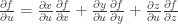
We continue our discussion of multivariate calculus. The first item here is the analogue of Chain Rule for the multivariate case. Suppose we have parameters f, u, v, x, y, z. Suppose {u, v} are independent parameters (in particular, the system is at least 2-dimensional), and assume that (i) we can write $x = x(u,v)$ , $y = y(u,v)$ and $z = z(u,v)$ as functions of {u, v}, (ii) we can write $f = f(x, y, z)$ as a function of x, y and z. This also means we can write f as a function of u and v. Upon perturbing the system, we get:

$\delta f \approx \delta x\left.\frac{\partial f}{\partial x}\right|_{y,z} + \delta y\left.\frac{\partial f}{\partial y}\right|_{x,z} + \delta z\left.\frac{\partial f}{\partial z}\right|_{x,y},$ and

$\delta f \approx \delta u\left.\frac{\partial f}{\partial u}\right|_v + \delta v\left.\frac{\partial f}{\partial v}\right|_u$ .

We wish to find a formula which expresses the second set of partial derivatives in terms of the first. To do that, we divide the first equation by $\delta u$ and obtain:

$\frac{\delta f}{\delta u} \approx \frac{\delta x}{\delta u}\left(\left.\frac{\partial f}{\partial x}\right|_{y,z}\right) + \frac{\delta y}{\delta u}\left(\left.\frac{\partial f}{\partial y}\right|_{x,z}\right) + \frac{\delta z}{\delta u}\left(\left.\frac{\partial f}{\partial z}\right|_{x,y}\right).$

If we maintain $\delta v = 0$ and let $\delta u \to 0$ , then the LHS converges to $\left.\frac{\partial f}{\partial u}\right|_v$ by definition. Taking the limit on the RHS also, we obtain:

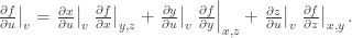
$\left.\frac{\partial f}{\partial u}\right|_v = \left.\frac{\partial x}{\partial u}\right|_v\left.\frac{\partial f}{\partial x}\right|_{y,z} + \left.\frac{\partial y}{\partial u}\right|_v\left.\frac{\partial f}{\partial y}\right|_{x,z} + \left.\frac{\partial z}{\partial u}\right|_v\left.\frac{\partial f}{\partial z}\right|_{x,y}.$

This is usually written in books as the simplified form: $\frac{\partial f}{\partial u} = \frac{\partial x}{\partial u}\frac{\partial f}{\partial x}+\frac{\partial y}{\partial u}\frac{\partial f}{\partial y} + \frac{\partial z}{\partial u}\frac{\partial f}{\partial z}$ , which is acceptable since the context is clear: the coordinate x is assumed to occur together with y and z, while u and v are always assumed to occur together. We left all the subscripts in our initial equation because we’re really trying to be careful here.

To remember the above formula, use the diagram:

Thus to compute $\frac{\partial f}{\partial u}$ we find all possible paths from f to u through the intermediate parameters {x, y, z} and take the sum of all terms, where each term is the product of the corresponding partial derivatives along the way.

Example 1. Suppose $f(x,y,z) = x^2 y^2 + yz^3 - xz$ and $x(u,v) = u^2 + v^2$ , $y(u,v) = 2uv$ , $z(u,v) = uv^3$ . Then

$\frac{\partial f}{\partial x} = 2xy^2 - z,\ \frac{\partial f}{\partial y}=2x^2 y+z^3, \ \frac{\partial f}{\partial z} = 3yz^2 - x$ .

Together with $\frac{\partial x}{\partial u} = 2u$ , $\frac{\partial y}{\partial u} = 2v$ and $\frac{\partial z}{\partial u} = v^3$ , we get the desired relation for $\frac{\partial f}{\partial u}$ which is convenient if we wish to calculate explicit values.

Example 2. Suppose we have polar coordinates $(x,y) = (r\cos \theta, r\sin \theta)$ . Then for any f = f(x, y),

$\frac{\partial f}{\partial r} = \frac{\partial f}{\partial x}\frac{\partial x}{\partial r} + \frac{\partial f}{\partial y}\frac{\partial y}{\partial r} = \cos\theta \frac{\partial f}{\partial x} + \sin\theta \frac{\partial f}{\partial y},$ – (1)

$\frac{\partial f}{\partial\theta} = \frac{\partial f}{\partial x}\frac{\partial x}{\partial\theta} + \frac{\partial f}{\partial y}\frac{\partial y}{\partial\theta} = -r\sin\theta \frac{\partial f}{\partial x} + r\cos\theta \frac{\partial f}{\partial y}$ – (2)

But if we wish to express $\frac{\partial f}{\partial x}$ and $\frac{\partial f}{\partial y}$ in terms of $\frac{\partial f}{\partial r}, \frac{\partial f}{\partial\theta}$ , then the equation $r\sin\theta \times (1) + \cos\theta\times (2)$ simplifies to: $r\sin\theta \frac{\partial f}{\partial r} + \cos\theta\frac{\partial f}{\partial\theta} = r\frac{\partial f}{\partial y}$ . A similar computation gives us an expression for $\frac{\partial f}{\partial x}$ . In short:

$\frac{\partial f}{\partial x} = \cos\theta \frac{\partial f}{\partial r}-\frac 1 r\sin\theta \frac{\partial f}{\partial\theta},\ \ \ \frac{\partial f}{\partial y} = \sin\theta \frac{\partial f}{\partial r} + \frac 1 r \cos\theta\frac{\partial f}{\partial\theta}.$

Higher Order Multivariate Derivatives

Recall that in the single-variable case, we can take successive derivatives of the function f(x) to obtain $\frac{df}{dx}$ , $\frac{d^2 f}{dx^2}$ , $\frac{d^3 f}{dx^3}$ etc. Let’s consider the multivariate case here.

Suppose {x, y, z, w} forms a set of coordinates. If we fix the values of y, z, and w then we can differentiate a function $f(x,y,z,w)$ with respect to x as many times as we please. Thus we write this as:

$\left.\frac{\partial^n f}{\partial x^n}\right|_{y,z,w} := \frac{d^n f}{dx^n}$ , keeping y, z, w constant.

For example, if $f(x,y,z,w) = x^3 y + xz^2 - w^4$ , then $\left.\frac{\partial^2 f}{\partial x^2}\right|_{y,z,w} = 6xy$ .

On the other hand, if we fix the values of z and w, then we can differentiate with respect to x first while keeping y constant, then with respect to y while keeping x constant. This is denoted by:

$\left.\frac{\partial^2 f}{\partial y \partial x}\right|_{z,w} := \left.\frac{\partial}{\partial y}\left(\left.\frac{\partial f}{\partial x} \right|_{y,z,w}\right)\right|_{x,z,w}.$

But one can also switch the order around: differentiate with respect to y first, then with respect to x. It turns out for the order doesn’t matter if the function is nice enough, i.e. we get:

$\left.\frac{\partial}{\partial y}\left(\left.\frac{\partial f}{\partial x}\right|_{y,z,w}\right)\right|_{x,z,w} = \left.\frac{\partial}{\partial x}\left(\left.\frac{\partial f}{\partial y}\right|_{x,z,w}\right)\right|_{y,z,w}.$

Here’s an intuitive (but non-rigourous) explanation of the reason. Since z, w are fixed throughout, let’s simplify our notation by denoting $g(x,y) = f(x,y,z,w)$ . Now consider a small perturbation $(x,y)\mapsto (x+\delta x, y+\delta y)$ and consider the following:

$\frac{g(x+\delta x, y+\delta y) - g(x, y+\delta y) - g(x+\delta x, y) + g(x,y)}{\delta x\cdot\delta y} = \frac{1}{\delta y}\left(\frac{g(x+\delta x, y+\delta y) - g(x, y+\delta y)}{\delta x} - \frac{g(x+\delta x, y) - g(x,y)}{\delta x}\right).$

If we let $\delta x\to 0$ with $\delta y$ constant, the two terms on the RHS converge to 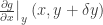$\left.\frac{\partial g}{\partial x}\right|_y (x, y+\delta y)$ and $\left.\frac{\partial g}{\partial x}\right|_y (x, y)$ respectively. If we now let $\delta y \to 0$ , the expression converges to $\left.\frac{\partial}{\partial y}\left(\left.\frac{\partial g}{\partial x}\right|_y\right)\right|_x$ . By symmetry, the equation also converges to $\left.\frac{\partial}{\partial x}\left(\left.\frac{\partial g}{\partial y}\right|_x\right)\right|_y$ if we switch the order of convergence. Since it shouldn’t matter whether we let $\delta x\to 0$ first then $\delta y\to 0$ or vice versa, the two derivatives are equal.

[ Warning: pathological examples where the two derivatives differ do exist! Such functions are explicitly forbidden in our consideration. ]

Example 3. Consider $f(x,y,z) = x^3 y + 3xz^2 - xy^4 z$ . Then the two derivatives are:

$\frac{\partial}{\partial x}\frac{\partial f}{\partial y} = \frac{\partial}{\partial x}(x^3 - 4xy^3 z) = 3x^2 - 4y^3 z$ ,

$\frac{\partial}{\partial y}\frac{\partial f}{\partial x} = \frac{\partial}{\partial y}(3x^2 y + 3z^2 - y^4 z) = 3x^2 - 4y^3 z$ .

Example 4. Consider rectilinear coordinates (x, y) and polar coordinates (r, θ), where the two are related via $(x, y) = (r\cos\theta, r\sin\theta)$ . We already know from example 2 that:

Let’s see if we can express the second derivatives with respect to {x, y} in terms of those with respect to {r, θ}. It may look horrid, but the calculations can be simplified by thinking of $\frac \partial{\partial x}$ as an operator, i.e. a function which takes functions to other functions! Thus we shall write:

$\frac{\partial}{\partial x} = \cos\theta \frac{\partial}{\partial r} - \frac {\sin\theta}r \frac{\partial}{\partial\theta}.$

So to get the second derivative in terms of x, we just apply the operator to itself:

$\frac{\partial^2}{\partial x^2} = \left(\cos\theta \frac{\partial}{\partial r} - \frac {\sin\theta}r \frac{\partial}{\partial\theta}\right)\left( \cos\theta \frac{\partial}{\partial r} - \frac {\sin\theta}r \frac{\partial}{\partial\theta}\right).$

Since the operators are all additive (an operator D is said to be additive if D(f + g) = Df + Dg for all functions f and g), we can use the distributive property to expand the RHS. Beware, though, that operators are in general not commutative; for example, by the product law we get:

$\frac{\partial}{\partial r}\left(\frac{\sin\theta}r \frac{\partial}{\partial\theta}\right) = \frac{\partial}{\partial r}\left(\frac{\sin\theta}r\right)\frac{\partial}{\partial\theta} + \frac{\sin\theta}{r} \frac{\partial^2}{\partial r\partial\theta} = -\frac{\sin\theta}{r^2}\frac{\partial}{\partial\theta} + \frac{\sin\theta}{r} \frac{\partial^2}{\partial r\partial \theta}.$

Now the reader has enough tools to verify the following:

$\frac{\partial^2}{\partial x^2} = \cos^2\theta \frac{\partial^2}{\partial r^2} + \frac{\sin^2\theta}{r^2} \frac{\partial^2}{\partial\theta^2} - \frac{\sin 2\theta}r \frac{\partial^2}{\partial r \partial\theta} + \frac {\sin 2\theta}{2r^2} \frac{\partial}{\partial \theta} + \frac{\sin^2\theta}{r} \frac{\partial}{\partial r}$ ,

$\frac{\partial^2}{\partial y^2} = \sin^2\theta \frac{\partial^2}{\partial r^2} + \frac{\cos^2\theta}{r^2} \frac{\partial^2}{\partial \theta^2} + \frac{\sin 2\theta}{r} \frac{\partial^2}{\partial r\partial\theta} - \frac{\sin 2\theta}{2r^2} \frac{\partial}{\partial \theta} + \frac{\cos^2\theta}{r} \frac{\partial}{\partial r}$ .

The case of $\frac{\partial^2}{\partial x\partial y}$ is left as an exercise for the reader.

Exercises

All hints are ROT-13 encoded to avoid spoilers.

Obligatory mechanical exercises: in each of the following examples, verify that , etc, via explicit computations.
1. $f(x, y) = \sin(x^2 + y^3)\exp(xy)$ .
2. $f(x,y,z) = \sin(xy) (x^3 z + y^2) \exp(z^3)$ .
If f = f(x, y), and z = x + y, is there any relationship between $\frac{\partial f}{\partial x}$ , $\frac{\partial f}{\partial y}$ and $\frac{\partial f}{\partial z}$ ? [ Hint: Ner nyy guerr cnegvny qrevingvirf jryy-qrsvarq? ]
In 3-D space, we can define spherical coordinates $(r, \theta, \phi)$ which satisfies $x = r\sin\theta\cos\phi$ , $y = r\sin\theta\sin\phi$ , $z = r\cos\theta$ . For a function f = f(x, y, z), express the partial derivatives $\frac{\partial f}{\partial x}, \frac{\partial f}{\partial y}, \frac{\partial f}{\partial z}$ in terms of spherical coordinates.
Prove that there does not exist f(x, y) such that $\frac{\partial f}{\partial x} = x^2y + xy^2$ and $\frac{\partial f}{\partial y} = x^3 + x^2 y$ .
Given $(x, y) = (u^2 - v^2, 2uv)$ , for a function f(x, y), express $\frac{\partial f}{\partial x}$ and $\frac{\partial f}{\partial y}$ in terms of u and v, and the partial derivatives of f with respect to u and v.
Find all points on the curve $x^3 + 2y^3 - 3xy = 1$ where the curve is tangent to a circle centred at the origin (see diagram below for a sample circle). You may use wolframalpha to numerically obtain the values.
(*) (Legendre transform) Suppose we have a 2-dimensional system with (non-independent) parameters u, v, w. Define the parameter $f = \left.\frac{\partial u}{\partial v}\right|_w$ . Explicitly write down a new parameter g in terms of u, v, w, f such that $\left.\frac{\partial g}{\partial f}\right|_w = -v$ . [ Hint: lbh pna pbzcyrgryl vtaber bar bs gur cnenzrgref. ]
(*) For a set of coordinates {x, t} in the plane, the differential equation $\frac{\partial^2 f}{\partial x^2} = \frac{\partial^2 f}{\partial t^2}$ is called the 1-dimensional wave equation. Find all general solutions of this equation. [ Hint: fhofgvghgr gur gjb inevnoyrf ol gur fhz naq gur qvssrerapr. ]

(Sample answer for question 6)

Posted in Notes | Tagged calculus, chain rule, higher order derivatives, legendre transform, multivariate, polar coordinates, spherical coordinates, wave equation | Leave a comment

Thinking Infinitesimally – Multivariate Calculus (I)

Posted on April 15, 2012 by limsup

[ Background required: some understanding of single-variable calculus, including differentiation and integration. ]

The object of this series of articles is to provide a rather different point-of-view to multivariate calculus, compared to the conventional approach in calculus texts. The typical approach is to take a (say) 2-variable function F(x, y) and consider the partial derivatives by differentiating with respect to one variable and keeping the other constant. E.g. for $F(x,y) = x^3 - 2xy^2$ , keeping y constant gives $\frac{\partial F}{\partial x} = 3x^2 - 2y^2$ and keeping x constant gives $\frac{\partial F}{\partial y} = -4xy$ . When it comes to implicit differentiation of multivariate functions, confusion can ensue. For example, we all know that $\frac{dy}{dx} \frac{dx}{dy} = 1$ in single-variable calculus. What about $\frac{\partial y}{\partial x}\frac{\partial z}{\partial y}\frac{\partial x}{\partial z}$ in the multivariate case?

In fact, the equation as it stands doesn’t even make sense without proper context. The correct statement is that on a two-dimensional surface in 3-space, we can fix one variable (say z) and take the partial derivative of another (say y) with respect to the last (x), giving the value $\left.\frac{\partial y}{\partial x}\right|_z$ . Then we ask for the value of:

$\left.\frac{\partial y}{\partial x}\right|_z \cdot \left.\frac{\partial z}{\partial y}\right|_x \cdot \left.\frac{\partial x}{\partial z}\right|_y$ .

This is now a sensible question, but it’s still hard even if you’ve had some experience with multivariate calculus. Things can get much worse in thermodynamics, where we often fix different variables before taking the partial derivatives. Hopefully, our approach here will help the reader to answer such questions with little difficulty.

Warning: the level of rigour in this series of articles is rather low, since we’re more concerned on the underlying intuition and heuristics.

Let’s begin.

First, we imagine a system with some set of real-valued parameters a, b, c, x, y, z. We shall give no preference to any of the parameters – rather, we will consider all of them at one go. Not all of these parameters are independent. For example, we may have x = ab, in which case {a, b, x} is not an independent set of parameters.

Now, we shall perturb the system by a little, and assume that the system is sufficiently well-behaved. By that, we mean that the change in each parameter will be small:

$a \mapsto a + \delta a, \ b \mapsto \delta b, \ c \mapsto \delta c, \ldots$

Note that we’re not changing the system slowly and measuring the rate of change with respect to time. One can certainly imagine including time as a parameter for some systems, but it will not be awarded extra favours in any manner. In other words, time may be a parameter, but just one out of many (side note: this point-of-view is essential in special relativity, where it is critical in dispelling countless seemingly paradoxical scenarios).

In most reasonable systems, we can specify at each point (by point, we mean a state whereby the system takes specific values for the parameters $(a_0, b_0, \dots)$ ) some independent parameters $x_1, x_2, \dots, x_n$ , such that:

no matter how we perturb the parameters $x_1, x_2, \dots, x_n$ , as long as the perturbation is small, there is a corresponding change in the system for that;
all the remaining parameters can be expressed as a function of $x_1, x_2, \dots, x_n$ .

We will then call this an n-parameter system. Thus, we can express any nearby point uniquely with $x_1, x_2, \dots, x_n$ . We reiterate that this set of n parameters is not unique, or even preferred. Such a set of n parameters is called a coordinate system.

Example 1. Consider the unit circle on the Cartesian plane, centred at origin. A system would correspond to a point on this circle. This gives a 1-parameter system. Let’s look at parameters $x, y, x^2, x^2 + y^2$ . Now, on almost all points on the circle, we can pick x as a coordinate and express the remaining parameters as a function in x. E.g. $y = \sqrt{1-x^2}$ for points on the upper semicircle and $y = -\sqrt{1-x^2}$ for those on the lower semicircle. We say “almost all” points because we can’t do this at the points (-1, 0) and (+1, 0). By the same token, we can use y as a coordinate on all points of the circle except (0, -1) and (0, +1).

Example 2. Consider the surface of a unit sphere $x^2 + y^2 + z^2 = 1$ . This is a 2-parameter system. For most points on the sphere, we can simply pick coordinates {x, y}. Where does this fail?

The above examples illustrate two points (pun unintended, seriously).

Not all sets of n parameters can form a coordinate system, even if we focus on only a point. For example, the parameter $x^2 + y^2$ in example 1 will forever be 1 (i.e. forever alone).
We don’t expect a single coordinate system $\{x_1, \dots, x_n\}$ to work for all points of the system. If you’re lucky, maybe, but don’t bet on it.
What we do expect is that, at every point P of the system, we can pick a set of n coordinates depending on the point, such that all points near P can be parametrised by these n coordinates uniquely. When we move from P to Q, we may have to switch to a new set of coordinates though.

Oh, and we expect n to be constant throughout the system, and it’s called the dimension of the system. E.g. for the plane we have rectilinear coodinates $(x,y)$ and polar coordinates $(r,\theta)$ , so the system is 2-dimensional. For 3-D space, we have rectilinear coordinates $(x,y,z)$ , cylindrical coordinates $(\rho,\theta, z)$ and spherical coordinates $(r,\phi,\theta)$ .

Now we can define partial differentiation for an n-parameter system (i.e. of dimension n). To fix ideas, let’s go back to the example of the system with parameters a, b, c, x, y, z, where we assume n=3 and pick coordinates {b, c, y}. We can fix any n-1 = 2 coordinates, say {b, y}, and vary the third (c) ever so slightly and delicately to give $c + \delta c$ . Now for any other parameter, say a, we consider the corresponding change $a \mapsto a + \delta a$ . The partial derivative is then defined by:

$\left.\frac{\partial a}{\partial c}\right|_{b,y} = \lim_{\delta c \to 0} \frac{\delta a}{\delta c},$ keeping b and y fixed.

In any sufficiently nice system, this limit exists. If there’s only one coordinate, then there’s no other parameter to fix so we can just write $\frac{da}{dc}$ for the above.

Most books usually write $\frac{\partial f}{\partial x}$ or something like that, without mentioning which other parameters have been fixed. That’s because f was usually defined as f(x, y, z), so there’s already an intrinsic set of coordinates. Here, we must warn the reader that if we fix different variables, the outcome may be different. Specifically, if we have coordinates {b, c, y} and {b, c, z}, then:

$\left.\frac{\partial a}{\partial c}\right|_{b,y} \ne \left.\frac{\partial a}{\partial c}\right|_{b,z}$

in general. But if the set of coordinates is obvious from the context, one can leave out the subscripts {b, y} or {b, z}.

Example 3. Consider the set of points on the plane. If we pick coordinates {x, y}, then the function z = 2x+y has partial derivative $\left.\frac{\partial z}{\partial x}\right|_y = 2$ . On the other hand, if we pick coordinates {x, w} with w = x+y, then z = x+w so we get the partial derivative $\left.\frac{\partial z}{\partial x}\right|_w = 1$ .

Now, comes the critical question.

What if we fix coordinate b, and perturb the remaining two coordinates $c\mapsto c+\delta c$ , $y \mapsto y +\delta y$ ? What’s the corresponding change in $a\mapsto a+\delta a$ ?

By definition of partial derivative, we can approximate:

$a(c+\delta c, y + \delta y) - a(c, y+\delta y) \approx \delta c \left.\frac{\partial a}{\partial c}\right|_y (c, y+\delta y).$

And next, $a(c, y+\delta y) - a(c,y)\approx \delta y \left.\frac{\partial a}{\partial y}\right|_y(c, y)$ . If we assume the partial derivatives are continuous, then we can further approximate:

$\left.\frac{\partial a}{\partial c}\right|_y (c, y+\delta y) \approx \left.\frac{\partial a}{\partial c}\right|_y(c,y)$ .

Putting it all together we obtain:

$\delta a = a(c + \delta c, y+\delta y) - a(c,y) \approx \delta c\left.\frac{\partial a}{\partial c}\right|_y + \delta y\left.\frac{\partial a}{\partial y}\right|_c.$

Example 4. Back to our first example of finding $F(x, y) = x^3 - 2xy^2$ . Then we have $\delta F \approx \left.\delta x\frac{\partial F}{\partial x}\right|_y + \left.\delta y\frac{\partial F}{\partial y}\right|_x = (3x^2 - 2y^2)\delta x + (-4xy)\delta y$ . In particular, at the point (x, y) = (2, 3), we have $\delta F \approx -6\delta x - 24\delta y$ . If we substitute concrete values δx = 0.00017, and δy = 0.00025, we get δF = -0.0070206 and -6 δx – 24 δy = -0.00702. Close enough.

If we plot this as a surface in 3-D space, then at the point (2, 3, -28) on the surface $z = F(x,y)$ , the plane which is tangent to the surface at the point is given by:

$(z + 28) = -6(x-2) - 24(y-3).$

Example 5. For the equation in example 3, consider the point (x, y) = (2, 3) as above. Let’s find the direction with the steepest angle of ascent/descent. For a slight perturbation δx and δy in x and y, consider the length of this difference: $\epsilon = \sqrt{(\delta x)^2 + (\delta y)^2}$ . The steepest direction is the one where δz is maximal across all fixed ε.

From linear algebra, we can rewrite $\delta z \approx (-6, -24)\cdot (\delta x, \delta y)$ via inner product, which as we recall is $\sqrt{6^2 + 24^2} \epsilon \cos\theta$ where θ is the angle between (-6, -24) and (δx, δy). Since ε is fixed, the climb is steepest when θ = 0, i.e. in the direction (-6, -24), or (1, 4).

The following 3D-graph and contour are plotted by wolframalpha:

At the point (2, 3), the diagram is consistent with our calculation, that (1, 4) is the direction of steepest ascent/descent.

In summary, for a surface plotted by z = f(x, y), the direction of steepest ascent/descent is precisely that of $(\frac {\partial f}{\partial x}, \frac{\partial f}{\partial y})$ . [ Notice I’ve stopped indicating which parameters are fixed; the context is clear. ] We usually denote this by:

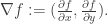
$\nabla f := (\frac{\partial f}{\partial x}, \frac{\partial f}{\partial y}).$

More generally, if we have n independent coordinates $x_1, \dots, x_n$ and $f = f(x_1, \dots, x_n)$ is a function of these coordinates, then we define:

$\nabla f := (\frac{\partial f}{\partial x_1}, \frac{\partial f}{\partial x_2}, \dots, \frac{\partial f}{\partial x_n})$ ,

which is a vector of length n.

Example 6. Consider the set of points on the curve defined implicitly by g(x, y) = 0. How do we compute $\frac{dy}{dx}$ at a point? Now, if we perturb the point by $(x, y) \mapsto (x + \delta x, y + \delta y)$ on the curve, then the resulting change δg = 0. On the other hand, since 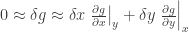$0 \approx \delta g \approx \delta x \left.\frac{\partial g}{\partial x}\right|_y + \delta y \left.\frac{\partial g}{\partial y}\right|_x$ , this gives:

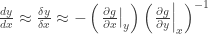$\frac{dy}{dx} \approx \frac{\delta y}{\delta x} \approx - \left(\left.\frac{\partial g}{\partial x}\right|_y\right) \left(\left.\frac{\partial g}{\partial y}\right|_x\right)^{-1}$ .

But you’ve seen this before: it’s just implicit differentiation. E.g. for the curve defined by $x^3 + y^3 - 3xy = 1$ , we let $g(x, y) = x^3 + y^3 - 3xy - 1$ , thus giving $\left.\frac{\partial g}{\partial x}\right|_x = 3x^2 - y^2$ and $\left.\frac{\partial g}{\partial y}\right|_x = 3y^2 - 3x$ . So:

$\frac{dy}{dx} = \frac{x^2 - y}{y^2 - x}$ .

Example 7. Let’s answer the question we posed at the beginning: on a 2-parameter system where the coordinate system can be {x, y}, {y, z} or {z, x}, what’s the value of:

$\left.\frac{\partial y}{\partial x}\right|_z \cdot \left.\frac{\partial z}{\partial y}\right|_x \cdot \left.\frac{\partial x}{\partial z}\right|_y$ ?

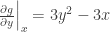One plausible method is to fix a coordinate system {x, y} and consider z = z(x, y) as a function in terms of these coordinates. But to preserve the symmetry, let’s consider the more general case where the three parameters are related by the equation $g(x,y,z) = 0$ . So when we perturb the system, we get $x\mapsto x+\delta x$ , $y\mapsto y+\delta y$ , $z\mapsto z+\delta z$ . All these happen while g remains constant, so:

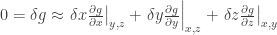$0 = \delta g \approx \left.\delta x\frac{\partial g}{\partial x}\right|_{y,z} + \left.\delta y\frac{\partial g}{\partial y}\right|_{x,z} + \left.\delta z\frac{\partial g}{\partial z}\right|_{x,y}$ . (#)

[ Note: in taking these three partial derivatives, we’re no longer on the 2-parameter system any more. Rather, we’re examining a larger system where g can vary, i.e. a 3-parameter system with coordinates {x, y, z}. ]

To compute $\left.\frac{\partial y}{\partial x}\right|_z$ we need to fix z, i.e. substitute $\delta z = 0$ in equation (#). This gives $0 \approx \left.\delta x\frac{\partial g}{\partial x}\right|_{y,z} + \left.\delta y\frac{\partial g}{\partial y}\right|_{x,z}$ . So, we have:

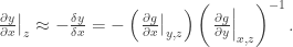
$\left.\frac{\partial y}{\partial x}\right|_z \approx -\frac{\delta y}{\delta x} = -\left(\left.\frac{\partial g}{\partial x}\right|_{y,z}\right) \left(\left.\frac{\partial g}{\partial y}\right|_{x,z}\right)^{-1}.$

By rotational symmetry, we also get similar expressions for $\left.\frac{\partial z}{\partial y}\right|_x$ and $\left.\frac{\partial x}{\partial z}\right|_y$ . So the overall product is -1. ♦

Possible topics coming up: chain law, vector calculus, jacobian, multivariate integration, differential forms, calculus of variations (where we have to contend with infinite-dimensioned systems!). But no guarantees though…

Exercises

Mechanical computations: find the partial derivatives of fwith respect to each of the coordinates.
1. $f(x, y) = x^3 + y^4 - 3x^2 y^2 - 4xy + 2x$ .
2. $f(x, y) = \cos(x^3) \sin(x^2 + \exp(y))$ .
3. $f(x, y, z) = \exp(-x - y^2 - z^3)$ .
More mechanical computations: find all the partial derivatives , … etc, on the surface defined by g(x, y, z) = 0.
1. $g(x, y, z) = x^4 y - y^2 z^2 + 3xz - 4z^3 - 5$ .
2. $g(x, y, z) = \cos(x^2 + y^3) - \sin(x + z^2) + \frac 1 2$ .
Consider the surface defined by and pick the point P = (2, 1, 0).
1. Find the direction of steepest descent/ascent at P.
2. Bob would like to walk from P while remaining exactly at sea level (z = 0). Find all possible directions for him to start walking.
Find the minimum value of the multivariate quadratic equation $f(x, y, z) = 5x^2 + 5y^2 + 3z^2 + 2xy - 6yz - 6xz + 4x - 4y$ for real x, y, z. [ Note: there’s no need to take the 2nd derivative. ]
A 2-dimensional surface in 4-space is given by the intersection of $x^4 + y^4 - 2z^4 + 2w^4 - xyzw = 1$ and $x^3 - y^2 - z + 2yz + w^3 = 2$ . Calculate the plane tangent to the surface at (1, 1, 1, 1).
On a 3-parameter system, what can we say about the product $\left.\frac{\partial w}{\partial x}\right|_{y,z} \times \left.\frac{\partial x}{\partial y}\right|_{w,z} \times \left.\frac{\partial y}{\partial z}\right|_{w,x} \times \left.\frac{\partial z}{\partial w}\right|_{x,y}$ ?
Intuition check. A system has parameters a, b, c, d. Upon some slight perturbation, we get corresponding parameters a+δa, b+δb, c+δc, d+δd which always satisfies $b^2\delta a + 4c \delta b - 3d \delta a = 0$ . Assuming no other infinitesimal relations exist among these parameters, what can we say about the dimension of the system (the number of parameters in a coordinate system)?

Posted in Notes | Tagged calculus, differentiation, intermediate, multivariate, partial differentiation | Leave a comment

17	18	19	20	21	22	23	24	25	26	27	28	29	30	31	32	33
*2	0	*1	0	*1	0	*1	0	*1	*2	*3	*2	*3	*2	*3	*2	*3

17	18	19	20	21	22	23	24	25	26	27	28	29	30	31	32	33
*2	0	*1	0	*1	0	*1	0	*1	*2	*3	*2	*3	*2	*3	*2	*3

Lesson 7

Hackenbush

Integers

Games With Value 1/2

Simplification (I)

More Fractions

Simplicity Rule

Proof of Simplicity Rule

In a Nutshell

Exercises

Lesson 6

General Combinatorial Game Theory

Domineering

Definition

Example

Addition of Games

Negative of Games

The Zero Game

Sum of a Game and Its Negative

Comparison Between Games

Application to Impartial Games

In a Nutshell

Exercises

Lesson 5

Nim’s Island

Winning Positions

Winning Strategy

Exercises

Some Notes

Lesson 4

Kayles

Sum of Two Games

Solving Kayles

Playing Kayles

Exercises

Lesson 3

Nim Value

Why Does It Work?

Example

Exercises

Lesson 2

Binary Representation

Solving Nim

Example

Playing Nim

The XOR Operation

Exercises

Lesson 1

Course Requirements

Square Game

Sieving Method

Remoteness

Exercises

Recent Posts

Archives

Categories

Meta

Pages

17	18	19	20	21	22	23	24	25	26	27	28	29	30	31	32	33
*2	0	*1	0	*1	0	*1	0	*1	*2	*3	*2	*3	*2	*3	*2	*3