
Chain Rule for Multivariate Calculus
We continue our discussion of multivariate calculus. The first item here is the analogue of Chain Rule for the multivariate case. Suppose we have parameters f, u, v, x, y, z. Suppose {u, v} are independent parameters (in particular, the system is at least 2-dimensional), and assume that (i) we can write 


We wish to find a formula which expresses the second set of partial derivatives in terms of the first. To do that, we divide the first equation by 

If we maintain 


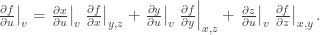
This is usually written in books as the simplified form: 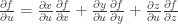
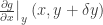
To remember the above formula, use the diagram:

Thus to compute 
Example 1. Suppose 
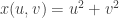


Together with 


Example 2. Suppose we have polar coordinates 


But if we wish to express 


Higher Order Multivariate Derivatives
Recall that in the single-variable case, we can take successive derivatives of the function f(x) to obtain 


Suppose {x, y, z, w} forms a set of coordinates. If we fix the values of y, z, and w then we can differentiate a function 

For example, if 

On the other hand, if we fix the values of z and w, then we can differentiate with respect to x first while keeping y constant, then with respect to y while keeping x constant. This is denoted by:

But one can also switch the order around: differentiate with respect to y first, then with respect to x. It turns out for the order doesn’t matter if the function is nice enough, i.e. we get:

Here’s an intuitive (but non-rigourous) explanation of the reason. Since z, w are fixed throughout, let’s simplify our notation by denoting 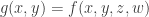


If we let 


[ Warning: pathological examples where the two derivatives differ do exist! Such functions are explicitly forbidden in our consideration. ]
Example 3. Consider 


Example 4. Consider rectilinear coordinates (x, y) and polar coordinates (r, θ), where the two are related via 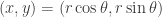
Let’s see if we can express the second derivatives with respect to {x, y} in terms of those with respect to {r, θ}. It may look horrid, but the calculations can be simplified by thinking of $\frac \partial{\partial x}$ as an operator, i.e. a function which takes functions to other functions! Thus we shall write:
So to get the second derivative in terms of x, we just apply the operator to itself:

Since the operators are all additive (an operator D is said to be additive if D(f + g) = Df + Dg for all functions f and g), we can use the distributive property to expand the RHS. Beware, though, that operators are in general not commutative; for example, by the product law we get:

Now the reader has enough tools to verify the following:


The case of 
![]()
Exercises
All hints are ROT-13 encoded to avoid spoilers.
- Obligatory mechanical exercises: in each of the following examples, verify that
,
etc, via explicit computations.
.
.
- If f = f(x, y), and z = x + y, is there any relationship between
? [ Hint: Ner nyy guerr cnegvny qrevingvirf jryy-qrsvarq? ]
- In 3-D space, we can define spherical coordinates
which satisfies
,
,
. For a function f = f(x, y, z), express the partial derivatives
in terms of spherical coordinates.
- Prove that there does not exist f(x, y) such that
and
.
- Given
, for a function f(x, y), express
- Find all points on the curve
where the curve is tangent to a circle centred at the origin (see diagram below for a sample circle). You may use wolframalpha to numerically obtain the values.
- (*) (Legendre transform) Suppose we have a 2-dimensional system with (non-independent) parameters u, v, w. Define the parameter
. Explicitly write down a new parameter g in terms of u, v, w, f such that
. [ Hint: lbh pna pbzcyrgryl vtaber bar bs gur cnenzrgref. ]
- (*) For a set of coordinates {x, t} in the plane, the differential equation
is called the 1-dimensional wave equation. Find all general solutions of this equation. [ Hint: fhofgvghgr gur gjb inevnoyrf ol gur fhz naq gur qvssrerapr. ]
 (Sample answer for question 6)
