Thinking Infinitesimally – Multivariate Calculus (I)

[ Background required: some understanding of single-variable calculus, including differentiation and integration. ]

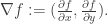
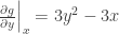
The object of this series of articles is to provide a rather different point-of-view to multivariate calculus, compared to the conventional approach in calculus texts. The typical approach is to take a (say) 2-variable function F(x, y) and consider the partial derivatives by differentiating with respect to one variable and keeping the other constant. E.g. for $F(x,y) = x^3 - 2xy^2$ , keeping y constant gives $\frac{\partial F}{\partial x} = 3x^2 - 2y^2$ and keeping x constant gives $\frac{\partial F}{\partial y} = -4xy$ . When it comes to implicit differentiation of multivariate functions, confusion can ensue. For example, we all know that $\frac{dy}{dx} \frac{dx}{dy} = 1$ in single-variable calculus. What about $\frac{\partial y}{\partial x}\frac{\partial z}{\partial y}\frac{\partial x}{\partial z}$ in the multivariate case?

In fact, the equation as it stands doesn’t even make sense without proper context. The correct statement is that on a two-dimensional surface in 3-space, we can fix one variable (say z) and take the partial derivative of another (say y) with respect to the last (x), giving the value $\left.\frac{\partial y}{\partial x}\right|_z$ . Then we ask for the value of:

$\left.\frac{\partial y}{\partial x}\right|_z \cdot \left.\frac{\partial z}{\partial y}\right|_x \cdot \left.\frac{\partial x}{\partial z}\right|_y$ .

This is now a sensible question, but it’s still hard even if you’ve had some experience with multivariate calculus. Things can get much worse in thermodynamics, where we often fix different variables before taking the partial derivatives. Hopefully, our approach here will help the reader to answer such questions with little difficulty.

Warning: the level of rigour in this series of articles is rather low, since we’re more concerned on the underlying intuition and heuristics.

Let’s begin.

First, we imagine a system with some set of real-valued parameters a, b, c, x, y, z. We shall give no preference to any of the parameters – rather, we will consider all of them at one go. Not all of these parameters are independent. For example, we may have x = ab, in which case {a, b, x} is not an independent set of parameters.

Now, we shall perturb the system by a little, and assume that the system is sufficiently well-behaved. By that, we mean that the change in each parameter will be small:

$a \mapsto a + \delta a, \ b \mapsto \delta b, \ c \mapsto \delta c, \ldots$

Note that we’re not changing the system slowly and measuring the rate of change with respect to time. One can certainly imagine including time as a parameter for some systems, but it will not be awarded extra favours in any manner. In other words, time may be a parameter, but just one out of many (side note: this point-of-view is essential in special relativity, where it is critical in dispelling countless seemingly paradoxical scenarios).

In most reasonable systems, we can specify at each point (by point, we mean a state whereby the system takes specific values for the parameters $(a_0, b_0, \dots)$ ) some independent parameters $x_1, x_2, \dots, x_n$ , such that:

no matter how we perturb the parameters $x_1, x_2, \dots, x_n$ , as long as the perturbation is small, there is a corresponding change in the system for that;
all the remaining parameters can be expressed as a function of $x_1, x_2, \dots, x_n$ .

We will then call this an n-parameter system. Thus, we can express any nearby point uniquely with $x_1, x_2, \dots, x_n$ . We reiterate that this set of n parameters is not unique, or even preferred. Such a set of n parameters is called a coordinate system.

Example 1. Consider the unit circle on the Cartesian plane, centred at origin. A system would correspond to a point on this circle. This gives a 1-parameter system. Let’s look at parameters $x, y, x^2, x^2 + y^2$ . Now, on almost all points on the circle, we can pick x as a coordinate and express the remaining parameters as a function in x. E.g. $y = \sqrt{1-x^2}$ for points on the upper semicircle and $y = -\sqrt{1-x^2}$ for those on the lower semicircle. We say “almost all” points because we can’t do this at the points (-1, 0) and (+1, 0). By the same token, we can use y as a coordinate on all points of the circle except (0, -1) and (0, +1).

Example 2. Consider the surface of a unit sphere $x^2 + y^2 + z^2 = 1$ . This is a 2-parameter system. For most points on the sphere, we can simply pick coordinates {x, y}. Where does this fail?

The above examples illustrate two points (pun unintended, seriously).

Not all sets of n parameters can form a coordinate system, even if we focus on only a point. For example, the parameter $x^2 + y^2$ in example 1 will forever be 1 (i.e. forever alone).
We don’t expect a single coordinate system $\{x_1, \dots, x_n\}$ to work for all points of the system. If you’re lucky, maybe, but don’t bet on it.
What we do expect is that, at every point P of the system, we can pick a set of n coordinates depending on the point, such that all points near P can be parametrised by these n coordinates uniquely. When we move from P to Q, we may have to switch to a new set of coordinates though.

Oh, and we expect n to be constant throughout the system, and it’s called the dimension of the system. E.g. for the plane we have rectilinear coodinates $(x,y)$ and polar coordinates $(r,\theta)$ , so the system is 2-dimensional. For 3-D space, we have rectilinear coordinates $(x,y,z)$ , cylindrical coordinates $(\rho,\theta, z)$ and spherical coordinates $(r,\phi,\theta)$ .

Now we can define partial differentiation for an n-parameter system (i.e. of dimension n). To fix ideas, let’s go back to the example of the system with parameters a, b, c, x, y, z, where we assume n=3 and pick coordinates {b, c, y}. We can fix any n-1 = 2 coordinates, say {b, y}, and vary the third (c) ever so slightly and delicately to give $c + \delta c$ . Now for any other parameter, say a, we consider the corresponding change $a \mapsto a + \delta a$ . The partial derivative is then defined by:

$\left.\frac{\partial a}{\partial c}\right|_{b,y} = \lim_{\delta c \to 0} \frac{\delta a}{\delta c},$ keeping b and y fixed.

In any sufficiently nice system, this limit exists. If there’s only one coordinate, then there’s no other parameter to fix so we can just write $\frac{da}{dc}$ for the above.

Most books usually write $\frac{\partial f}{\partial x}$ or something like that, without mentioning which other parameters have been fixed. That’s because f was usually defined as f(x, y, z), so there’s already an intrinsic set of coordinates. Here, we must warn the reader that if we fix different variables, the outcome may be different. Specifically, if we have coordinates {b, c, y} and {b, c, z}, then:

$\left.\frac{\partial a}{\partial c}\right|_{b,y} \ne \left.\frac{\partial a}{\partial c}\right|_{b,z}$

in general. But if the set of coordinates is obvious from the context, one can leave out the subscripts {b, y} or {b, z}.

Example 3. Consider the set of points on the plane. If we pick coordinates {x, y}, then the function z = 2x+y has partial derivative $\left.\frac{\partial z}{\partial x}\right|_y = 2$ . On the other hand, if we pick coordinates {x, w} with w = x+y, then z = x+w so we get the partial derivative $\left.\frac{\partial z}{\partial x}\right|_w = 1$ .

Now, comes the critical question.

What if we fix coordinate b, and perturb the remaining two coordinates $c\mapsto c+\delta c$ , $y \mapsto y +\delta y$ ? What’s the corresponding change in $a\mapsto a+\delta a$ ?

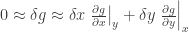
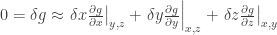
By definition of partial derivative, we can approximate:

$a(c+\delta c, y + \delta y) - a(c, y+\delta y) \approx \delta c \left.\frac{\partial a}{\partial c}\right|_y (c, y+\delta y).$

And next, $a(c, y+\delta y) - a(c,y)\approx \delta y \left.\frac{\partial a}{\partial y}\right|_y(c, y)$ . If we assume the partial derivatives are continuous, then we can further approximate:

$\left.\frac{\partial a}{\partial c}\right|_y (c, y+\delta y) \approx \left.\frac{\partial a}{\partial c}\right|_y(c,y)$ .

Putting it all together we obtain:

$\delta a = a(c + \delta c, y+\delta y) - a(c,y) \approx \delta c\left.\frac{\partial a}{\partial c}\right|_y + \delta y\left.\frac{\partial a}{\partial y}\right|_c.$

Example 4. Back to our first example of finding $F(x, y) = x^3 - 2xy^2$ . Then we have $\delta F \approx \left.\delta x\frac{\partial F}{\partial x}\right|_y + \left.\delta y\frac{\partial F}{\partial y}\right|_x = (3x^2 - 2y^2)\delta x + (-4xy)\delta y$ . In particular, at the point (x, y) = (2, 3), we have $\delta F \approx -6\delta x - 24\delta y$ . If we substitute concrete values δx = 0.00017, and δy = 0.00025, we get δF = -0.0070206 and -6 δx – 24 δy = -0.00702. Close enough.

If we plot this as a surface in 3-D space, then at the point (2, 3, -28) on the surface $z = F(x,y)$ , the plane which is tangent to the surface at the point is given by:

$(z + 28) = -6(x-2) - 24(y-3).$

Example 5. For the equation in example 3, consider the point (x, y) = (2, 3) as above. Let’s find the direction with the steepest angle of ascent/descent. For a slight perturbation δx and δy in x and y, consider the length of this difference: $\epsilon = \sqrt{(\delta x)^2 + (\delta y)^2}$ . The steepest direction is the one where δz is maximal across all fixed ε.

From linear algebra, we can rewrite $\delta z \approx (-6, -24)\cdot (\delta x, \delta y)$ via inner product, which as we recall is $\sqrt{6^2 + 24^2} \epsilon \cos\theta$ where θ is the angle between (-6, -24) and (δx, δy). Since ε is fixed, the climb is steepest when θ = 0, i.e. in the direction (-6, -24), or (1, 4).

The following 3D-graph and contour are plotted by wolframalpha:

At the point (2, 3), the diagram is consistent with our calculation, that (1, 4) is the direction of steepest ascent/descent.

In summary, for a surface plotted by z = f(x, y), the direction of steepest ascent/descent is precisely that of $(\frac {\partial f}{\partial x}, \frac{\partial f}{\partial y})$ . [ Notice I’ve stopped indicating which parameters are fixed; the context is clear. ] We usually denote this by:

$\nabla f := (\frac{\partial f}{\partial x}, \frac{\partial f}{\partial y}).$

More generally, if we have n independent coordinates $x_1, \dots, x_n$ and $f = f(x_1, \dots, x_n)$ is a function of these coordinates, then we define:

$\nabla f := (\frac{\partial f}{\partial x_1}, \frac{\partial f}{\partial x_2}, \dots, \frac{\partial f}{\partial x_n})$ ,

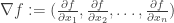
which is a vector of length n.

Example 6. Consider the set of points on the curve defined implicitly by g(x, y) = 0. How do we compute $\frac{dy}{dx}$ at a point? Now, if we perturb the point by $(x, y) \mapsto (x + \delta x, y + \delta y)$ on the curve, then the resulting change δg = 0. On the other hand, since $0 \approx \delta g \approx \delta x \left.\frac{\partial g}{\partial x}\right|_y + \delta y \left.\frac{\partial g}{\partial y}\right|_x$ , this gives:

$\frac{dy}{dx} \approx \frac{\delta y}{\delta x} \approx - \left(\left.\frac{\partial g}{\partial x}\right|_y\right) \left(\left.\frac{\partial g}{\partial y}\right|_x\right)^{-1}$ .

But you’ve seen this before: it’s just implicit differentiation. E.g. for the curve defined by $x^3 + y^3 - 3xy = 1$ , we let $g(x, y) = x^3 + y^3 - 3xy - 1$ , thus giving $\left.\frac{\partial g}{\partial x}\right|_x = 3x^2 - y^2$ and $\left.\frac{\partial g}{\partial y}\right|_x = 3y^2 - 3x$ . So:

$\frac{dy}{dx} = \frac{x^2 - y}{y^2 - x}$ .

Example 7. Let’s answer the question we posed at the beginning: on a 2-parameter system where the coordinate system can be {x, y}, {y, z} or {z, x}, what’s the value of:

$\left.\frac{\partial y}{\partial x}\right|_z \cdot \left.\frac{\partial z}{\partial y}\right|_x \cdot \left.\frac{\partial x}{\partial z}\right|_y$ ?

One plausible method is to fix a coordinate system {x, y} and consider z = z(x, y) as a function in terms of these coordinates. But to preserve the symmetry, let’s consider the more general case where the three parameters are related by the equation $g(x,y,z) = 0$ . So when we perturb the system, we get $x\mapsto x+\delta x$ , $y\mapsto y+\delta y$ , $z\mapsto z+\delta z$ . All these happen while g remains constant, so:

$0 = \delta g \approx \left.\delta x\frac{\partial g}{\partial x}\right|_{y,z} + \left.\delta y\frac{\partial g}{\partial y}\right|_{x,z} + \left.\delta z\frac{\partial g}{\partial z}\right|_{x,y}$ . (#)

[ Note: in taking these three partial derivatives, we’re no longer on the 2-parameter system any more. Rather, we’re examining a larger system where g can vary, i.e. a 3-parameter system with coordinates {x, y, z}. ]

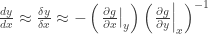
To compute $\left.\frac{\partial y}{\partial x}\right|_z$ we need to fix z, i.e. substitute $\delta z = 0$ in equation (#). This gives $0 \approx \left.\delta x\frac{\partial g}{\partial x}\right|_{y,z} + \left.\delta y\frac{\partial g}{\partial y}\right|_{x,z}$ . So, we have:

$\left.\frac{\partial y}{\partial x}\right|_z \approx -\frac{\delta y}{\delta x} = -\left(\left.\frac{\partial g}{\partial x}\right|_{y,z}\right) \left(\left.\frac{\partial g}{\partial y}\right|_{x,z}\right)^{-1}.$

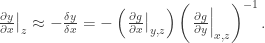
By rotational symmetry, we also get similar expressions for $\left.\frac{\partial z}{\partial y}\right|_x$ and $\left.\frac{\partial x}{\partial z}\right|_y$ . So the overall product is -1. ♦

Possible topics coming up: chain law, vector calculus, jacobian, multivariate integration, differential forms, calculus of variations (where we have to contend with infinite-dimensioned systems!). But no guarantees though…

Exercises

Mechanical computations: find the partial derivatives of fwith respect to each of the coordinates.
1. $f(x, y) = x^3 + y^4 - 3x^2 y^2 - 4xy + 2x$ .
2. $f(x, y) = \cos(x^3) \sin(x^2 + \exp(y))$ .
3. $f(x, y, z) = \exp(-x - y^2 - z^3)$ .
More mechanical computations: find all the partial derivatives , … etc, on the surface defined by g(x, y, z) = 0.
1. $g(x, y, z) = x^4 y - y^2 z^2 + 3xz - 4z^3 - 5$ .
2. $g(x, y, z) = \cos(x^2 + y^3) - \sin(x + z^2) + \frac 1 2$ .
Consider the surface defined by and pick the point P = (2, 1, 0).
1. Find the direction of steepest descent/ascent at P.
2. Bob would like to walk from P while remaining exactly at sea level (z = 0). Find all possible directions for him to start walking.
Find the minimum value of the multivariate quadratic equation $f(x, y, z) = 5x^2 + 5y^2 + 3z^2 + 2xy - 6yz - 6xz + 4x - 4y$ for real x, y, z. [ Note: there’s no need to take the 2nd derivative. ]
A 2-dimensional surface in 4-space is given by the intersection of $x^4 + y^4 - 2z^4 + 2w^4 - xyzw = 1$ and $x^3 - y^2 - z + 2yz + w^3 = 2$ . Calculate the plane tangent to the surface at (1, 1, 1, 1).
On a 3-parameter system, what can we say about the product $\left.\frac{\partial w}{\partial x}\right|_{y,z} \times \left.\frac{\partial x}{\partial y}\right|_{w,z} \times \left.\frac{\partial y}{\partial z}\right|_{w,x} \times \left.\frac{\partial z}{\partial w}\right|_{x,y}$ ?
Intuition check. A system has parameters a, b, c, d. Upon some slight perturbation, we get corresponding parameters a+δa, b+δb, c+δc, d+δd which always satisfies $b^2\delta a + 4c \delta b - 3d \delta a = 0$ . Assuming no other infinitesimal relations exist among these parameters, what can we say about the dimension of the system (the number of parameters in a coordinate system)?