Note: this article is noticeably more difficult than the previous instalments. The reader is advised to be completely comfortable with generating functions before proceeding.
We’ve already seen how generating functions can be used to solve some combinatorial problems. The nice thing is that even if a sequence has no nice closed form, generating functions allow us to efficiently compute a large number of terms in the sequence. With modern computers, such computations are often a cakewalk.
Here, we shall look at a different type of generating functions. Given a sequence  , let us define:
 .
.
This is called the exponential generating function (EGF) of the sequence an. Here’re some easy examples.
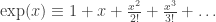
- The EGF for an = 1 is given by
 ; that’s why there’s an “exponential” attached to the name.
- The EGF for an = n! is given by
 .
.
- The EGF for an = rn is given by
 .
.
When do we use this and not the standard generating function? Generally speaking, the EGF is useful for counting the number of combinatorial objects for a labeled set, while the standard generating function is useful for an unlabeled set. Here’s why, roughly.
- Suppose, to get a structure A on n identical balls, we need to split the set of n balls into two disjoint subsets and impose structure B on the first subset, and structure C on the second subset. Under this assumption, if an (resp. bn, cn) denotes the number of structures of type A (resp. B, C) on the set of n balls, then we have
 , since we need to consider the case where the first subset has 0, 1, 2, …, or n balls.
- Now consider the same problem, except that the n identical balls are replaced by the set {1, 2, …, n}. To count an, suppose we choose a k-subset
 ; there are
  possible choices for S. Then we impose a structure B on S; there are bk ways of doing this. And finally, we choose a structure C on the remaining
  ; there are cn-k ways of doing this. This gives
  , or
, or  , thus their EGFs multiply to give the final EGF.
Without further delay, let’s look at some concrete examples.

Problem 1. Find the number of functions f : {1, 2, …, n} → {1, 2, …, r}.
Solution. Any beginning student of combinatorics knows the solution: rn. But let’s derive this using EGF. Corresponding to each f, we take the inverse image  which are subsets of {1, 2, …, n}. Let
  ; then we get a partition of {1, 2, …, n} into r disjoint subsets:

Hence, to find a function f, we only need to state an ordered partition into r subsets (“ordered” here means that swapping S1 and S2 changes the partition). If r is fixed, and an denotes the number of f, then the EGF for (an) is the product of r copies of the sequence (1, 1, 1, … ):
 .
.
But the coefficient of  in
in  is
is  , so we get the result
  as expected. ♦
Problem 2. Find the number of surjections f : {1, 2, …, n} → {1, 2, …, r}, where r ≤ n.
Solution. We now have the partition  , where each
  is non-empty. So the corresponding EGF for each term is now the EGF of (0, 1, 1, 1, …), which is
 .
.
Hence, if we fix r and let an denote the number of surjections f, then the EGF for an is  . ♦
. ♦
Let’s consider small values of r:
- r = 2 : EGF =
 , so
, so  .
.
- r = 3 : EGF =
 , so
, so  .
.
- r = 4 :
 .
.
- …
Now the astute reader can easily write down the general formula.
Problem 3. Consider all possible functions f : {1, 2, …, n} → {1, 2, …, s}. What is the expected size of the image of f ?
Solution. Fix n and s. Let  be the number of f whose image has size r. If we consider the case im(f) = {1, 2, …, r}, then the number of such f is n! times the coefficient of in . Hence, is exactly
  times this number. So we need to look at:
 (*)
(*)
Thus it really suffices to simplify  . This can be achieved by differentiating the binomial expansion:

 .
.
So our sum simplifies to  . Upon substituting
  , the sum (*) simplifies to
  . This gives
  . Dividing by the total number of possible functions (
 ), the mean image size is
  , which is very close to s-1 for large s. ♦
Exercise 1. Find the number of r-letter words you can form with the letters ‘a’, ‘b’ and ‘c’, where ‘a’ occurs an odd number of times and ‘b’ occurs an even number of times.
Exercise 2. The Stirling number of the second kind  is the number of partitions of {1, 2, …, n} into r disjoint non-empty subsets. Write down an expression for by computing its EGF or otherwise. Also write down an expression for the Bell number
  , which is the number of partitions of {1, 2, …, n}. [ Note: the partitions here are unordered, i.e.
  and
and  are considered identical partitions. ]
Exercise 3. (Comtet’s square). Let  be the number of ways to partition {1, 2, …, n} such that (i) the number of parts is X; and (ii) the size of each part is Y, where X, Y are elements of {“unrestrained”, “even”, “odd”}. Find the EGF for . Since there’re 9 possible ordered pairs for (X, Y), you should get 9 answers in all.
Throughout this section, we shall require the reader to be somewhat acquainted with the concept of permutations. A permutation of order n is a bijective map from {1, 2, …, n} to itself. For example, we can express a permutation of order 9 via the following diagram:

Such a permutation p would map 1 to 3, 2 to 5, 3 to 9, … . Or one can also express the same permutation in the form of cycles:

which is clearer and one immediately knows how the successive powers  act on the numbers 1, …, 9. For example, since the three cycles have lengths 1, 3, and 5, the smallest n for which
  is n = lcm(1,3,5) = 15. We say that the order of the permutation is 15.
An element i for which p(i) = i is called a fixed point of the permutation p. In the above example, the only fixed point is 4.
Problem 4. Let be the number of permutations p of {1, 2, …, n} such that  . [ Such a permutation is called an involution. ] Find the exponential generating function of .
Proof. If we write p as a product of cycles as above, then p is an involution iff all the cycles have lengths 1 or 2. If there are exactly r cycles (where r is fixed), then the number of permutations has exponential generating function in n given by:  , right?
No! Since swapping the cycles has no discernible effect on the permutation (e.g. (1, 2)(4, 5)3 = (1, 2)3(4, 5)), we should divide it by r!. Hence, we should look at  instead. Summing over all r, we get:

This allows us to express as a sum:
![a_n = \sum_{k=0}^{[n/2]} \frac{n!}{2^k k! (n-2k)!}.](https://s0.wp.com/latex.php?latex=a_n+%3D+%5Csum_%7Bk%3D0%7D%5E%7B%5Bn%2F2%5D%7D+%5Cfrac%7Bn%21%7D%7B2%5Ek+k%21+%28n-2k%29%21%7D.&bg=ffffff&fg=333333&s=0&c=20201002) ♦
♦
Problem 5. Find the number of permutations p of {1, 2, …, n}, where p is a product of an even number of disjoint cycles.
Solution. As in the previous problem, we consider the case of r cycles. Given the set {1, 2, …, s}, how many cycles p of length s can we form? To answer that, for any such cycle we can start from 1 and obtain a unique sequence of s-1 numbers via  which is a permutation of {2, 3, …, s}. Hence the number is (s-1)!, which gives the EGF:

To find the number of p where p is a product of r cycles, we have to take n! times the coefficient of in  . [ As before, the factor of
  is included since swapping cycles does not change the permutation. ] Hence to find the EGF for , we sum over all even r:

where  is the hyperbolic cosine function. Hence the above simplifies to
  . In conclusion:
- When n = 0,
 .
.
- When n = 1,
 (obviously!).
- When n ≥ 2,
 . ♦
. ♦
Note : considering how nice the answer is, one naturally wonders if there is a nice combinatorial argument for this. There is, actually. If p is any permutation of {1, 2, …, n}, where  , we compose it with (1, 2) to give
  . If 1 and 2 belong to the same cycle of p, the composed permutation q would split them up into two cycles; conversely, if 1 and 2 belong to disjoint cycles, then q merges the two cycles into one. The proof is left as an exercise.
But that’s how things are; one often discovers such patterns through heavy machinery before finding a simpler combinatorial proof.
Exercise 4. A derangement is a permutation without a fixed point (i.e. for all i, p(i) ≠ i). Prove that the number of derangements of {1, 2, …, n} is  .
.
Exercise 5. Prove that the number of permutations p of {1, 2, …, 2n} having only even cycle lengths, is given by  .
.
Exercise 6. Generalise the above two problems as follows. Let  be two subsets. We wish to enumerate the number of permutations of {1, 2, …, n} for which
- the number of cycles is an element of B; and
- the length of each cycle is an element of A.
Prove that the EGF of the sequence can be expressed in the form  , where α(x) (resp. β(x)) is a power series which depends solely on A (resp. B). Find these power series.
Exercise 7. Prove that the number of permutations of {1, 2, …, n} containing an even number of even-length cycles is exactly  when n ≥ 2. For extra challenge, go for two proofs: one combinatorial and one via EGF.
Exercise 8. Prove that the expected number of cycles of a random permutation of {1, 2, …, n} is given by  , which is very close to log(n).
Exercise 9. (New: bonus question)* A permutations p of {1, 2, …, n} is said to be alternating if p(1) < p(2), p(2) > p(3), p(3) < p(4), p(4) > p(5), etc. If f(x) denotes the EGF of the number of alternating permutations of {1, 2, …, n}, find a relation between f(x) and its derivative f’(x). Hence prove that f(x) = tan(x).
This concludes our discussion of EGF. Though the article is rather long, we’ve barely scratched the surface of what generating functions are capable of. In particular, one can look at combinatorial species, where an equality not only establishes that  , but an actual bijection between the associated combinatorial structures. The best way to understand this is via category theory, but that’s really another story for another day.


 , where
  are positive integers. We are interested in counting the number of partitions of n, which is denoted by p(n).
 , we place
  dots on a row, evenly spaced apart and starting from a left margin; then
  dots on the second row, again evenly spaced apart and starting from the same left margin, etc. For example, for the two partitions 18 = 6+5+3+3+1 = 4+4+4+3+1+1+1, we have the corresponding Young diagrams.

 , where p(0) is taken to be 1 (there’s just one way to partition 0: i.e. don’t do anything). Now, instead of looking at the individual parts in a partition, we can count the number of 1’s, the number of 2’s etc and represent this by a tuple
  of non-negative integers such that
  . For example, the above two Young diagrams correspond to tuples (1, 0, 2, 0, 1, 1) and (3, 0, 1, 3) respectively. This gives:
 .
. is given by:
 .
. or
or  . Comparing the coefficient of
  for the sequence is
 .
. we get:
 such that (i)
  gets at least one ball, and (ii) while any balls remain, each successive urn receives at least as many balls as all previous urns combined. On the other hand, let b(n) be the number of partitions of n into powers of 2, possibly with repeated terms. Prove that a(n) = b(n). E.g. if n = 6, then:
 be the generating function of the sequence b(n). From the above argument, it’s clear that:
 .
. on both sides then gives us:
 ;
; .
. , suppose we distribute 2n+1 balls among the urns. Look at the last urn: the number of balls in this urn must be more than the number of balls in all prior urns; for if it were equal, then the total number of balls would be even (contradiction). By removing 1 ball from the last urn, we get a bijection between the distributions of 2n+1 balls and those of 2n balls.
 , consider a distribution of 2n balls. If the last urn has as many balls as all prior urns combined, then removing the last urn gives us a distribution of n balls. If it has more, then removing one ball gives a distribution of 2n-1 balls. You can easily check that we obtain bijections in both cases. This completes the proof. ♦
 . Prove that the number of partitions of n into m
  into at most m parts.
 , where
  is a 3rd root of unity, satisfying
  . If you’re not familiar with complex numbers, just note that
  is 2 (resp. -1) if n is divisible (resp. not divisble) by 3. ]
 where
where  ,
,  ,
,  ,
,  . Prove that the generating function of c(n) is
  .
. .
. , when expanded, has very few non-zero entries. To be specific:
 .
. .
.
 terms above. If you know programming, you can now use Python to calculate up to p(1000) easily. 🙂
 be the mass of particle i;
 be respectively the x-, y– and z-components of the velocity of i.
 .
. . Next, since the gas is homogeneous, the pressure on the top/bottom wall is given by P. To compute P in terms of the microscopic state, consider a single particle hitting the wall and having an elastic collision.
 . Since the height of the container is L, the particle takes time
  to hit the top wall again. So on average, the change in momentum per unit time is given by:

 .
.

 which is linear in N.
 so the entropy is given by
  . Applying Stirling’s approximation for factorials, we can also see that if U/N = p is constant, then S is linear in N, but since we won’t need this fact, there’s no necessity to dwell on it any more.
 , where i = 1, 2, …, N. The microstate of the entire system then corresponds to a point in the 6N-dimensional space which, to put it mildly, is a staggeringly huge space. Since the total energy
  is constant, we’re looking at a (6N-1)-dimensional hypersurface D defined by:
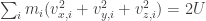 . (*)
. (*) , written as
  for short, and count the “number” of accessible configurations subjected to the constraint that U is constant. Since our space is continuous, by “number” we really mean volume.
 (i = 1, 2, … , N) can occur anywhere in a space of volume V. Here D’ is the (3N-1)-dimensional subspace defined by the equation (*) above. This is a huge hyper-ellipsoidal surface which we’ll approximate with a cube (if you feel perturbed by this, we will justify it at the end of the article: basically the approximation just changes the entropy by a constant multiple of N):
 for a constant λ which is independent of N and U. This shows that:
 ,
, .
. and
and  , there is no change in the state of the system even on a microscopic scale. So in counting the number of states, we really should divide
  by a factor of N!.
 possible states and thus entropy
  . Upon releasing the middle wall, there should be no change in the total entropy since the two gases are identical. But if we assume all the particles are distinct, then by pairing up particles in the two chambers (there’re effectively N particles in each, despite the micro-fluctuations) we gain a factor of 2N in the total number of states, which contributes an additional factor to the entropy. This is known as Gibbs paradox. To offset it, we assume particles which are interchanged do not contribute to additional states.
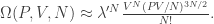
 so this gives
 ,
, has become one of the founding principles of statistical physics. [ Boltzmann’s story had a bitter-sweet ending to it – his theory eventually gained acceptance and the formula
  was
was  as a measure in computing the volume. What if we had multiplied this measure by a constant factor? Specifically, if say we had chosen
  instead, then the whole measure would be multiplied by a factor of
  . The net effect this has on the entropy is
  which is absorbed by the kN term.
 with a cube instead. To justify this, let m and M be the minimum and maximum of the mi‘s. If M/m is not too huge, we can bound the expression
  ; and for the reverse inequality, if
  then
then  . Once again, we only affect the entropy by a constant multiple of N.
 , then
 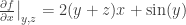 . ]
. ] and
and  . But is there any physical meaning to F other than a mere symbolic convenience? Well, yes. There’re at least two ways of looking at it.
 .
. .
. , which is the negation of the change in free energy. Hence one can envisage converting the free energy into work.
 .
.

 ;
; ;
; .
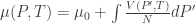
.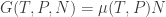 for some positive
  . This is called the chemical potential of the system. This parameter is clearly intensive.
 .
. . Simplifying this relation, we obtain:
 and N by N and N0 respectively, we see that t(N) is of the form:
  for some constant k. Hence, the formula for entropy is now:
 , where v= V/N.
 the graph has two turning points. The state (P, V) of the material is unstable between these two points. For if we reduce the volume a little by compressing it, then the decrease in pressure causes it to be compressed further; conversely, if we expand it a little, then the increase in pressure will continue to expand it. Indeed, within this region the material is in a mixture of liquid and gaseous state (we say it is in vapour-liquid equilibrium for the pure system).
 (here, P doesn’t increase monotonically over the integration region!). Recall that v = V/N. The result of the integral is hence the difference of the areas of the two shaded regions below. [ Note: this is non-trivial, do take a minute to figure out what the integration means over a non-monotonically increasing variable. ]
 , i.e. the two shaded regions have the same area. This is known as Maxwell construction, which gives us the condition for which the liquid and gaseous state can coexist. Note that the region is wider than the interval between the two turning points. The remaining intervals correspond to meta-stable states; these states can exist if we prepare the material sufficiently slowly and carefully but they’re highly delicate and unstable.
 . This approaches the critical point, beyond which there is no clear distinction between the liquid and gaseous states.

 . The corresponding pressure and volume at the critical point are
  and
and  .
. , constant N, whose ideal gas temperature is
  . Next we subject it to the following cycle:
 . Expand it to
  .
. . Measure the temperature and write it as
  .
. . Contract it to
  .
. since N is constant, and during adiabatic transformation, we have
  . If we look at the state of the gas throughout the entire transformation, we get the following P–V graph:
 from the hotter source during the first step, and a deposit of heat
  into the colder source during the third step, i.e. it is a reversible heat engine! Let’s calculate
  by writing out the equations relating the state parameters.
 since this is isothermal;
 since this is adiabatic;
 since this is isothermal;
 since this is adiabatic.
 , or
, or  .
.
 . Hence the ratios do match:
 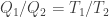 , so the ideal gas temperature scale is consistent with the thermodynamic temperature up to a scaling factor.
 sequentially, and takes in heat
  from the heat source
  . Here,
  . Equality holds if and only if the entire process is reversible.
 extracted equal to zero? ]
 from T;
 .
. along the path is independent of the process we pick, as long as it is reversible. Thus we can define a state parameter S such that
  , or in differential format,
  . This is the entropy of the system, which is well-defined up to an additive constant.
 to
to  , assuming N is fixed for now. What better choice than to pick parts of the Carnot cycle?
 , where Q is the total amount of heat pumped in. Since the temperature of the system remains constant, so is the internal energy (remember: ideal gas!) and thus all heat is used to do work, i.e.
  since P = TN/V. This happens when
  .
. since dQ = 0 throughout (the very definition of adiabatic). This happens when
  .
.
 .
. . This gives the more commonly known variant of the second law of thermodynamics: the entropy of an adiabatically sealed system tends to increase. However, we now see that this is actually a consequence – in fact, without Clausius or Kelvin Law, we wouldn’t be able to define a total ordering on the set of temperatures, let alone talk about heat engines or define entropy.
 while the colder area gains entropy
  . Thus, if we only look at the union of these two heat sources, the change in entropy is
  .
. , the entropy of the system also tends to 0. In particular, the third law enables us to find the “additive constant” for the formula of entropy.
 . If we only know the initial and final states (P, V, N) and (P’, V’, N), we can’t evaluate the integral without knowing the entire path.
 which is the version normally taught in JCs (in Singapore).
 . This is not hard to solve:
 is called the efficiency of the heat engine. To motivate this definition, imagine a mechanical engine which taps into a hot pool of gas, performs work, and loses the remaining energy to the environment (at temperature T2). The work done by the engine is useful since it can be converted to other forms of mechanical work, while the energy lost to the environment is wasted.
 . Equality holds if and only if F is also reversible. [ In particular, this implies that the efficiency of a reversible heat engine is as good as it gets. ]
 which is equivalent. Approximate
  by a rational number M/N, where M and N are positive integers. Thus it suffices to show
  , or
, or  . Let’s perform some iterations of the above heat engines: N times of F, followed by M times of the reverse of E.
 while the heat extracted from the hot source is
  , all of which is converted to work! By Kelvin Law, the work done cannot be positive, so we have
  as desired.
 , which is the reciprocal of the rate of wastage. It follows that if
  , then from the following diagram:
 to the temperature source
  , with the difference converted to work. But this is precisely the work of a heat engine for
  . [ Note: one subtle assumption is that we can tune F to take in an exact amount of heat
  when
when  for
for  . More generally, we shall define
  and
and  if
if  . Under this new definition, we see that for any temperatures
  , the reversible heat engine will extract heat
  , we now have (regardless of the temperature ordering):
 ;
; ;
; .
. and define
  . The above 3 relations then tell us
  for any two temperatures. So the only function that really matters for reversible heat engines is a single parameter g. We shall define this as our temperature scale.
 and
and  .
.
 , where v = V/N. Notice that the ideal gas equation is the limiting case of van der Waal’s equation where a = b = 0. [ Van der Waal’s equation assumes that particles have positive size and have mutually attractice / repulsive forces, hence the difference. But we digress. ]


 while preserving the order of the variables. For example, if n = 4, we have 5 possible expressions:
 for the number of such expressions; the slightly shifted index is so that we get a nice expression in
  . Using the technique of divide-and-conquer, it is not hard to obtain a recurrence relation in the sequence. Indeed, if we pick an expression with n+1 variables, it must be of the form: (expr1) * (expr2), where the two expressions have (say) i and n+1-i variables respectively, where i = 1, 2, …, n. Hence we have:
 ,
,  . (*)
. (*) . Then the coefficient of
  in
in  is precisely the expression on the right of (*). Hence we have:
 . For n > 1, the coefficient of
  =
=  .
. . Since the
  .
. :
:
 grid. We wish to count the number of paths from the southwest corner to the northeast along the edges of the grid which are (i) shortest, and (ii) remain below the line joining the southwest and northeast corner. E.g. when n=3, we have 5 possible paths:


 , then the series doesn’t converge except at x = 0, but it still makes sense to talk about the series purely in notational form. We shall call such a power series a formal power series.
 , where each
  is a real (or complex) number.
 without any loss of data. However, the power series notation appeals more to our intuition due to the definitions which are about to follow.
 be any two formal power series. Then their sum and product are power series defined respectively as follows:
 ,
,  ,
, and
and  .
. which fails to converge for any non-zero x. Despite this, we can consider f(x) as a formal power series and take its square:
  . Note that we can calculate any coefficient as we please, but there doesn’t seem to be a nice closed formula for the general coefficient.
 ,
,  ;
; ,
,  ;
; ;
; , the ‘1’ polynomial satisfies
  ;
; , then f or g is zero (this will prove to be important later).
 .
. ?
? . If
. If  . Now suppose we have already found
  ; in order to compute the next coefficient, we need
  , which gives:
 ‘s inductively from
  onwards. It follows quite easily from our definition that the resulting power series g satisfies
  .
. .
. ;
; ;
; (exercise: prove it, try to make use of the first two properties and avoid dealing with the explicit coefficients).
 .
. , one only needs to take the first n terms
  .
. ;
; ;
; ;
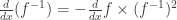
; (chain law of derivative).
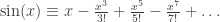 ;
; ;
; ;
; ;
; .
. .
. is a constant multiple of exp(x) (left as an exercise; hint:
  . Then its derivative satisfies, by the sum and product formulae:
 .
. satisfies
  and g is a multiple of exp(x). Since g has no constant term, it must be 0. ♦
 .
. and
and  , where
  . Use example 1. ♦
 .
. . It’s easy to show that any power series satisfying
  is a constant multiple of
  (left as an exercise). Hence, the derivative of f is:
 . Since the constant term of f is zero, we have f = 0.
 .
. satisfied by P and concluded that P can be obtained by the binomial expansion. While it’s true that the resulting binomial expansion does give Q such that
  , how do we conclude that
  ?
? . In order to derive this, we simplify
  . The fact that there are no non-zero zero divisors (#) then says R+S or R-S is zero.
 as follows.
 .
. , as an equality of formal power series. Hence we get
  .
. for some real constants a, b, r, s.
 . Obtain Binet’s formula.
 .
. is given by
  .
. ,
,  ?
? in closed form.
 and
and  and what they mean. Also, some examples / problems may require calculus. ]
 , one can write the polynomial
  in x. We shall call this polynomial the generating function for the sequence. This is useful when one needs to evaluate certain identities based on the
 .
.
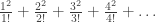
 we get the following combinatorial identity by looking at the coefficient of
  :
: .
. , we thus obtain, by looking at the coefficient of
  on both sides:
 is defined to be zero whenever i is not in the range 0, 1, …, n. In particular, if m = n = r, then using the equality
  we obtain:
 .
. ;
; , if you know complex numbers.
 .
. , simplify the sum:
 .
.
 , there is a unique non-negative real number R (or possibly +∞) such that:
 , then the series converges for x;
 , then the series does not converge for x.
 converges is x = 0.
 converges for all x < 1. In fact, you should know that this is
  .
. . We can apply l’Hôpital’s rule to the above formula to obtain R = 1. In fact, we can differentiate example 2 with respect to x to obtain:
 .
. be the Fibonacci sequence defined by
  and
and 
 . [ Exercise: prove it; hint: use
  . ] So the radius of convergence is
 .
. . Using the identity
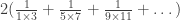
 . Hence,
  for all such x. In particular, when x=1/2, we obtain:
 . By bounding the value of n! (e.g. by using integration, as we
  . Thus, the radius of convergence is +∞ and the sequence
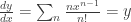 . To solve for y, we invert the derivative to obtain
  so
so  . Substituting x=0, y=1 gives us c=0. So in short:
 . Problem arises when we attempt to use the
  formula: since the even terms are zero while the odd terms are not, the limit does not exist! However, the main theorem still holds, i.e. the radius of convergence R must exist, regardless of whether the above limit does.
 , we get
 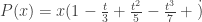 , we see that the bracketed term converges for |t|<1 and diverges for |t|>1. Hence, P(x) converges for |x|<1 and diverges for |x|>1, so the radius of convergence is 1.
 , we see that this power series is precisely the arc-tangent:
 .
. and the bracketed term is less than
  . So the power series does converge at x=1 and x=-1, and we get:
 .
. .
. ;
; ;
; .
. .
. .
.