Why Do We Need Eigenvalues and Eigenvectors?

[ Prerequisites : basic linear algebra, matrices and determinants. ]

Eigenvalues and eigenvectors are often confusing to students the first time they encounter them. This article attempts to demystify the concepts by giving some motivations and applications. It’s okay if you’ve never heard of eigenvectors / eigenvalues, since we will take things one step at a time here.

Note: all vectors are assumed to be column vectors here, and a matrix acts on a vector via left multiplication.

Consider the matrix $M = \begin{pmatrix} 3 & 1\\ 1 & 3\end{pmatrix}$ . We know mathematically what it does: it takes a (column) vector v = (x, y) to w = (3x+y, x+3y). But what’s the geometry behind it? If we take the circle C with radius 1 and centre at origin, then the matrix maps C to the ellipse C’ as follows:

(Image from wolframalpha.com)

As for how we obtained the equation $(3x-y)^2 + (3y-x)^2 = 64$ , that’s left as an exercise. 🙂 From the diagram, it should be clear that the matrix M “stretches” vectors along the diagonals. Specifically, let’s tilt our head 45° and pick the basis comprising of $v = (1, 1)$ and $w = (-1, 1)$ . Then we get $Mv = (4, 4) = 4v$ and $Mw = (-2, 2) = 2w$ . Since {v, w} forms a basis of the plane, we get:

$M(\alpha v + \beta w) = \alpha\cdot Mv + \beta\cdot Mw = (4\alpha)v + (2\beta)w.$

Thus geometrically, M behaves very much like the diagonal matrix $D=\begin{pmatrix} 4 & 0 \\ 0 & 2\end{pmatrix}$ . We will expound on this now: writing $Q = (v|w)$ , we get $MQ = (Mv|Mw) = (4v|2w) = QD$ , where D is the diagonal matrix above. Since {v, w} forms a basis, the matrix Q is invertible so:

$M = QDQ^{-1}$ .

More generally, we say that matrices M and N are similar if there exists an invertible matrix Q such that $M = QNQ^{-1}$ . For a given matrix M, the process of finding a similar diagonal matrix D is called diagonalisation. Generally, the fact that M is similar to a diagonal matrix can be useful, both conceptually and computation-wise.

Exercise 1 : if M and N are similar, as are M’ and N’, does that mean M+M’ and N+N’ are similar?

From $M = QDQ^{-1}$ we get $M^2 = (QDQ^{-1})(QDQ^{-1}) = QD^2Q^{-1}$ . More generally, one can show by induction that $M^n = QD^n Q^{-1}$ in general. This spells good news for us: since D is diagonal, its powers can be easily evaluated: $D^n = \begin{pmatrix} 4^n & 0 \\ 0 & 2^n\end{pmatrix}$ . Putting it all together with $Q^{-1} = \frac 1 2\begin{pmatrix} 1 & 1\\ -1 & 1\end{pmatrix}$ , we get a closed form:

$M^n = \frac 1 2\begin{pmatrix}1 & -1\\ 1 & 1\end{pmatrix} \begin{pmatrix}4^n & 0 \\ 0 & 2^n\end{pmatrix}\begin{pmatrix}1 & 1\\ -1 & 1\end{pmatrix} = \frac 1 2\begin{pmatrix}4^n + 2^n & 4^n - 2^n\\ 4^n-2^n & 4^n + 2^n\end{pmatrix}$ .

Example: Binet’s Formula

This is (yet) another derivation of Binet’s formula for the Fibonacci sequence: $F_0 = 0, F_1 = 1, F_{n+1} = F_n + F_{n-1}$ for $n\ge 1$ . If we consider the column vector $v_n = (F_{n+1}, F_n)$ , then the recurrence $F_{n+1} = F_n + F_{n-1}$ translates to the following matrix relation:

$\begin{pmatrix} 1 & 1\\ 1 & 0\end{pmatrix}\begin{pmatrix}F_n\\F_{n-1}\end{pmatrix} = \begin{pmatrix}F_{n+1}\\F_n\end{pmatrix}\implies \begin{pmatrix} 1 & 1\\ 1 & 0\end{pmatrix} v_{n-1} = v_n$ .

Thus, we get 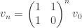$v_n = \begin{pmatrix} 1 & 1\\ 1 & 0\end{pmatrix}^n v_0$ . This strongly suggests diagonalising the matrix $A=\begin{pmatrix} 1 & 1 \\ 1 & 0\end{pmatrix}$ .

To do so, we need to find vectors v and w such that $Av = \lambda_1 v$ and $Aw = \lambda_2 w$ for some scalar values $\lambda_1, \lambda_2$ . Of course, v and w are non-zero vectors here, so this means the matrix $(A - \lambda_i\cdot I)$ (where i = 1, 2) maps some non-zero vector to zero. In other words, $\det(A - \lambda_i\cdot I) = 0$ . But we can expand via the determinant formula to obtain:

$\det(A - \lambda I) = 0 \implies \det\begin{pmatrix} 1-\lambda & 1 \\ 1 & -\lambda\end{pmatrix} = 0 \implies (1-\lambda)(-\lambda) - 1 = 0$ .

Solving for this quadratic equation we get $\lambda_1 = \frac{1+\sqrt{5}}2$ and $\lambda_2 = \frac{1-\sqrt{5}}2$ , which explain the terms in Binet’s formula. We’ll leave the rest to the reader.

More generally, if p(x) is any polynomial with real coefficients, then we can write 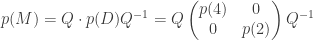$p(M) = Q\cdot p(D) Q^{-1} = Q\begin{pmatrix} p(4) & 0\\ 0 & p(2)\end{pmatrix}Q^{-1}$ . For example, if $p(x) = x^4 + 3x^2 - x + 1$ , then we have:

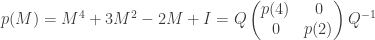
$p(M) = M^4 + 3M^2 - 2M + I = Q\begin{pmatrix} p(4) & 0 \\ 0 & p(2)\end{pmatrix}Q^{-1}$

and evaluate accordingly.

And why stop at polynomials? Why not infinite power series? Indeed, recall the Taylor expansion for the exponential function $e^x = \exp(x) = 1 + x + \frac{x^2}{2!} + \frac{x^3}{3!} + \dots$ . We can define it for matrices also: for any matrix M, let us write:

$\exp(M) = I + M + \frac{M^2}{2!} + \frac{M^3}{3!} + \dots$ .

Infinite sums are always rather pesky since we’re not sure if they converge. This is even more so for matrices. Fortunately, since we have the diagonalisation $M = QDQ^{-1}$ , we even know exactly what it converges to:

$I + M + \frac{M^2}{2!} + \frac{M^3}{3!} + \dots = Q\left(I + D + \frac{D^2}{2!} + \dots\right)Q^{-1} = Q\begin{pmatrix} 1 + 4 + \frac{4^2}{2!} +\dots & 0 \\ 0 & 1 + 2 + \frac{2^2}{2!} + \dots\end{pmatrix}Q^{-1} = Q\begin{pmatrix} e^4 & 0 \\ 0 & e^2\end{pmatrix}Q^{-1}$ .

Exercise 2. Prove that for any real numbers t and s, $\exp(tM) \exp(sM) = \exp((t+s)M)$ .

Exercise 3. Is it true that $\exp(A) \exp(B) = \exp(A+B)$ for any two matrices?

Exercise 4. Define cos(A) and sin(A) for an arbitrary matrix A. [ Hint: if you know complex numbers, there’s no need to write them in Taylor expansion. ] Is it true that $\cos^2(A) + \sin^2(A) = I$ for any matrix A? What about $\sin(A+B) = \sin A \cos B + \cos A \sin B$ ?

Clearly we can generalise the above discussion to n × n matrices in general. Specifically, let M be a square matrix. If there is a scalar λ and a non-zero vector v such that $Mv = \lambda v$ , then we say λ is an eigenvalue with corresponding eigenvector v.

Next, M is diagonalisable if we can write $M = QDQ^{-1}$ for some invertible matrix Q and diagonal matrix D. E.g. if M is a 4 × 4 matrix and we can diagonalise it as:

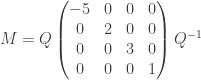$M = Q\begin{pmatrix} -5 & 0 & 0 & 0\\ 0 & 2 & 0 & 0\\ 0 & 0 & 3 & 0\\ 0 & 0 & 0 & 1\end{pmatrix}Q^{-1}$ ,

then we know that the general entries of $M^n$ can be written as a fixed linear combination of the powers (-5)ⁿ, 2ⁿ, 3ⁿ, 1ⁿ=1. In particular, when n is large, the absolute values of the entries are approximately a constant times 5ⁿ.

In short, if we know the largest eigenvalue λ of a matrix, then we can approximate the size of the entries of $M^n$ via a constant times $\lambda^n$ . For this reason, we have a special name for this value. The spectral radius of a matrix M is defined to be the largest |λ| among all eigenvalues λ of M.

As mentioned earlier, to diagonalise an n × n matrix M in general, we first write MQ = QD for some diagonal matrix D. If we break the matrix Q into column vectors $(v_1 | v_2 | \dots | v_n)$ , then this translates to:

$Mv_1 = \lambda_1 v_1,\ Mv_2 = \lambda_2 v_2, \dots, Mv_n = \lambda_n v_n$ ,

for some scalar values $\lambda_1, \lambda_2, \dots, \lambda_n$ . But this just means each $v_i$ is a non-zero vector satisfying $(M-\lambda_i I)v_i = 0$ so the matrix $M - \lambda_i I$ is singular for each i. This means the eigenvalues of M are precisely the values of λ such that $\det(M - \lambda I) = 0$ !

It turns out not all matrices are diagonalisable. But most of the time they are:

Theorem. If an n × n matrix M has n distinct eigenvalues (i.e. the equation $\det(M - \lambda I) = 0$ has no repeated root), then M is diagonalisable.

Proof. Let the n distinct eigenvalues be $\lambda_i$ , i = 1, 2, …, n. Each eigenvalue must have some corresponding eigenvector $v_i$ . Let $Q = (v_1 | v_2 | \dots | v_n)$ . The relation $M v_i = \lambda_i v_i$ then says $MQ = QD$ where D is the diagonal matrix with diagonal entries $\lambda_1, \lambda_2, \dots$ .

Thus, we only need to prove Q is invertible, or equivalently, that $v_1, v_2, \dots, v_n$ are linearly independent. To that end, suppose they are linearly dependent. We re-order the eigenvectors and eigenvalues and drop extraneous terms such that:

$c_1 v_1 + c_2 v_2 + \dots + c_k v_k = 0$

for some non-zero scalar values c_i and k ≤ n is as small as possible. Now let M act on both sides. Using the fact that $Mv_i = \lambda_i v_i$ , we get:

$c_1 \lambda_1 v_1 + c_2 \lambda_2 v_2 + \dots + c_k \lambda_k v_k = 0.$

Multiplying the first equation by $\lambda_1$ and taking the difference, we thus get an even shorter relation with smaller k. This contradicts the minimality of k. ♦

Thus, if one picks some random matrix with random entries, the result is almost certainly diagonalisable.

Exercse 5. Prove that the matrix $M =\begin{pmatrix} 2 & 1 \\ 0 & 2\end{pmatrix}$ is not diagonalisable. Write the entries of $M^n$ in closed form.

Why Do We Need Eigenvalues and Eigenvectors?

Leave a Reply Cancel reply

Recent Posts

Archives

Categories

Meta

Pages

Why Do We Need Eigenvalues and Eigenvectors?

Share this:

Like this:

Related

Leave a Reply Cancel reply

Recent Posts

Archives

Categories

Meta

Pages