Kinetic Theory, Entropy and Information Theory

This is really a continuation from the series “Thermodynamics for Mathematicians”. Our discussion then wasn’t quite complete without some justifications of the facts we used from kinetic theory of gases, in particular, we will figure out the constant c in the formula U = c·PV. At the end of this post, we will also relate the thermodynamic definition of entropy with the statistical entropy, which is the log of the number of configurations.

The fundamental assumption of kinetic theory is that an ideal gas comprises of molecules. Let’s not assume they’re identical for now, and instead label them via 1, 2, 3, … . Suppose they’re contained in a box with height L and base area A. Let:

$m_i$ be the mass of particle i;
$v_{x,i}, v_{y,i}, v_{z,i}$ be respectively the x-, y– and z-components of the velocity of i.

If we assume the internal energy U is given by the kinetic energy of these particles, then we get:

$U = \sum_i \frac 1 2 m_i (v_{x,i}^2 + v_{y,i}^2 + v_{z,i}^2) = \sum_i \frac 1 2 m_i v_{x,i}^2 + \sum_i \frac 1 2 m_i v_{y,i}^2 + \sum_i \frac 1 2 m_i v_{z,i}^2$ .

Assuming there’s no gravity effect, the three terms are identical by symmetry since nature has no preferred direction. We thus get: $U =\frac 3 2 \sum_i m_i v_{z,i}^2$ . Next, since the gas is homogeneous, the pressure on the top/bottom wall is given by P. To compute P in terms of the microscopic state, consider a single particle hitting the wall and having an elastic collision.

Hence, change in momentum of a single particle is $2m_i v_{z,i}$ . Since the height of the container is L, the particle takes time $2L/v_{z,i}$ to hit the top wall again. So on average, the change in momentum per unit time is given by:

$\frac{2m_i v_{z,i}} {2L/v_{z,i}} = m_i v_{z,i}^2/L.$

And that’s just one particle. The total force exerted on the top wall is the sum of all such terms. Hence, the pressure (force exerted per unit area) is given by

$P = \frac 1 A\sum_i m_i v_{z,i}^2/L = \frac 1 V \sum_i m_i v_{z,i}^2,$

where V is the volume of the container. Equating this formula with the earlier one, we get $U = \frac 3 2 PV$ .

[ Note: this section requires multivariate calculus and integration, of a very large number of dimensions! ]

Thus, the formula for adiabatic transformation of an ideal gas is:

$\left( \frac{P'}P\right) = \left(\frac{V'}V\right)^{-5/3}.$

And the formula for entropy of an ideal gas is:

$S(P, V, N) = N(\frac 3 2 \log P + \frac 5 2 \log \frac V N) + kN,$

where k is a constant we can’t know without delving into quantum mechanics (we’ll explain why later). Finally, we’ll explain how this ties in with statistical entropy. For this, we’ll need to define:

The statistical entropy (S) for a system subjected to certain constraints is the logarithm of the number of configurations (Ω) subjected to these constraints, assuming each configuration occurs with equal probability.

To fix ideas, one may imagine a finite number of possible configurations. For a concrete example suppose we have a huge table top filled with N coins, each of which is either a head or a tail. If the coin is fair, then there are Ω(N) = 2^N possible configurations occurring with equal probability, and statistical entropy is thus $S(N) = \log(2^N) = N\log 2$ which is linear in N.

Now suppose we add another constraint: that the number of heads is exactly U. Now the number of configurations is $\Omega(N, U) = C(N, U)$ so the entropy is given by $S(N, U) = \log C(N,U)$ . Applying Stirling’s approximation for factorials, we can also see that if U/N = p is constant, then S is linear in N, but since we won’t need this fact, there’s no necessity to dwell on it any more.

And how does the statistical entropy relate to the thermodynamic one?

To answer that, we look at the case of an ideal gas: we have to “count” the number of states with a given (P, V, N) and show that it’s logarithm is precisely the thermodynamic entropy.

Consider the position and velocity of each particle: $(x_i, y_i, z_i, v_{x,i}, v_{y,i}, v_{z,i})$ , where i = 1, 2, …, N. The microstate of the entire system then corresponds to a point in the 6N-dimensional space which, to put it mildly, is a staggeringly huge space. Since the total energy $U = \frac 1 2 \sum_i m_i (v_{x,i}^2 + v_{y,i}^2 + v_{z,i}^2)$ is constant, we’re looking at a (6N-1)-dimensional hypersurface D defined by:

$\sum_i m_i (v_{x,i}^2 + v_{y,i}^2 + v_{z,i}^2) = 2U$ . (*)

Now we partition the entire space into small blocks $\prod_{i=1}^N dx_i dy_i dz_i dv_{x,i} dv_{y,i} dv_{z,i}$ , written as $\prod_{i=1}^N d\mathbf{r}_i d\mathbf{v}_i$ for short, and count the “number” of accessible configurations subjected to the constraint that U is constant. Since our space is continuous, by “number” we really mean volume.

$\Omega(P, V, N) = \int_D 1 \cdot \prod_{i=1}^N d\mathbf{r}_i d\mathbf{v}_i = V^N \int_{D'} 1 \cdot\prod_{i=1}^N d\mathbf{v}_i,$

since each $\mathbf{r}_i$ (i = 1, 2, … , N) can occur anywhere in a space of volume V. Here D’ is the (3N-1)-dimensional subspace defined by the equation (*) above. This is a huge hyper-ellipsoidal surface which we’ll approximate with a cube (if you feel perturbed by this, we will justify it at the end of the article: basically the approximation just changes the entropy by a constant multiple of N):

$|v_{x_i}|, |v_{y,i}|, |v_{z,i}| \le \sqrt{2U/(6mN)},$

for a constant m which approximates m_i. The (hyper)volume of D’ is then given by $\lambda^N \sqrt{U/N}^{3N}$ for a constant λ which is independent of N and U. This shows that:

$\Omega(P, V, N) \approx \lambda^N V^N (U/N)^{3N/2} = \lambda'^N V^N (PV/N)^{3N/2}$ ,

which gives the statistical entropy:

$S(P, V, N) = \log \Omega(P, V, N) \approx N(\log V + \frac 3 2\log (V/N) + \frac 3 2 \log P) + kN$ .

This doesn’t quite match the thermodynamic entropy. What’s wrong?

Gibbs Paradox

The problem is that if we swap the states of two particles $(\mathbf{r}_i, \mathbf{v}_i)$ and $(\mathbf{r}_j, \mathbf{v}_j)$ , there is no change in the state of the system even on a microscopic scale. So in counting the number of states, we really should divide $\Omega$ by a factor of N!.

If you’re still not convinced, here’s a qualitative argument: consider the case where we have two identical bodies of gases with the same (P, V, N) separated by an adiabatic wall. Initially, the combined system has $\Omega = \Omega_1 \times \Omega_2$ possible states and thus entropy $S = S_1 + S_2$ . Upon releasing the middle wall, there should be no change in the total entropy since the two gases are identical. But if we assume all the particles are distinct, then by pairing up particles in the two chambers (there’re effectively N particles in each, despite the micro-fluctuations) we gain a factor of 2^N in the total number of states, which contributes an additional factor to the entropy. This is known as Gibbs paradox. To offset it, we assume particles which are interchanged do not contribute to additional states.

Thus, the correct number of states is

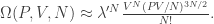
$\Omega(P, V, N) \approx \lambda'^N \frac{V^N (PV/N)^{3N/2}}{N!}.$

By Stirling’s approximation, we can take $\log N! \approx N(\log N - 1)$ so this gives

$S(P,V,N) \approx N(\frac 5 2\log(V/N) + \frac 3 2\log P) + kN$ ,

which matches the thermodynamic entropy.

To be honest, this process looks rather dubious. The fact that the coefficients match (3/2 and 5/2) is something of interest but appending a factor of -log(N!) seems forced. Indeed, Boltzmann faced a lot of opposition during his time in promoting his theory, which led to his depression and eventual suicide. After repeated success of the theory, however, the definition of $S = \log \Omega$ has become one of the founding principles of statistical physics. [ Boltzmann’s story had a bitter-sweet ending to it – his theory eventually gained acceptance and the formula $S = k \log W$ was carved onto his grave as remembrance for his great work. Here k is a scaling factor to convert our ideal gas temperature to Kelvin. ]

Finally, we take note of some choices we subtly made in computing S = S(P, V, N) and how changing them would affect S.

We specifically chose $d\mathbf{r}_i d\mathbf{v}_i$ as a measure in computing the volume. What if we had multiplied this measure by a constant factor? Specifically, if say we had chosen $d\mathbf{r}_i' = \alpha d\mathbf{r}_i$ instead, then the whole measure would be multiplied by a factor of $\alpha^N$ . The net effect this has on the entropy is $N\cdot \log \alpha$ which is absorbed by the kN term.
We had chosen to approximate the hyper-ellipsoid surface $\sum_i m_i(v_{x,i}^2 + v_{y,i}^2 + v_{z,i}^2) = 2U$ with a cube instead. To justify this, let m and M be the minimum and maximum of the m_i‘s. If M/m is not too huge, we can bound the expression $mv_x^2 \le m_i(v_x^2 + v_y^2 + v_z^2)$ ; and for the reverse inequality, if $|v_x|, |v_y|, |v_z| < K$ then $m_i(v_x^2 + v_y^2 + v_z^2) \le 3MK^2$ . Once again, we only affect the entropy by a constant multiple of N.

One thus sees and appreciates the amount of difficulty in computing the constant k in the formula for S. In particular, one must choose a specific measure when partitioning the large 6N-dimensional state space. What’s the right measure for us? The answer is supplied by quantum mechanics via Planck’s constant, which will give the Sackur-Tetrode equation, but that’s another story for another day.

Kinetic Theory, Entropy and Information Theory

Leave a Reply Cancel reply

Recent Posts

Archives

Categories

Meta

Pages

Kinetic Theory, Entropy and Information Theory

Share this:

Like this:

Related

Leave a Reply Cancel reply

Recent Posts

Archives

Categories

Meta

Pages