Commutative Algebra 47

Posted on May 5, 2020 by limsup

Minkowski Theory: Introduction

Suppose $K/\mathbb Q$ is a finite extension and $\mathcal O_K$ is the integral closure of $\mathbb Z$ in K.

In algebraic number theory, there is a classical method by Minkowski to compute the Picard group of $\mathcal O_K$ (note: in texts on algebraic number theory, this is often called the divisor class group; there is a slight difference between the two but for Dedekind domains they are identical).

We will only consider the simplest cases here to give readers a sample of the theory.

Minkowski’s Lemma.

If a measurable region $X\subseteq \mathbb R^2$ has area > 1, then there exist distinct $x, y\in X$ such that $x-y\in \mathbb Z^2$ .

Proof

Use the following picture:

minkowski_lemma

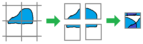
Since the area > 1, there exist two points which overlap in the unit square on the right. The corresponding $x,y\in X$ then give $x-y\in \mathbb Z^2$ . ♦

Minkowski’s Theorem.

Let $X\subseteq \mathbb R^2$ be a measurable region which is convex, symmetric about the origin and has area > 4. Then X has a lattice point other than the origin.

Proof

Take $\{\frac 1 2 x : x\in X\}$ , which has area > 1. By Minkowski’s lemma, there exist distinct $x, y\in X$ such that $\frac 1 2 x - \frac 1 2 y \in \mathbb Z^2$ . Since X is symmetric about the origin replace y by –y (so $x\ne -y$ ) to give $\frac 1 2 x + \frac 1 2 y \in \mathbb Z^2$ . And since X is convex, $x,y\in X \implies \frac 1 2 x + \frac 1 2 y \in X$ . Finally since $x \ne -y$ , $\frac 1 2 x + \frac 1 2 y$ is not the origin. ♦

By applying a linear transform to $\mathbb R^2$ we obtain the more useful version of Minkowski’s theorem.

Minkowski’s Theorem B.

Take a full lattice $\mathbb Z^2 \cong L \subset \mathbb R^2$ (i.e. discrete subgroup which spans $\mathbb R^2$ ). Taking a basis $(v_1, v_2)$ of L, we obtain a fundamental domain

$\{ \alpha_1 v_1 + \alpha_2 v_2 : 0 \le \alpha_1, \alpha_2 < 1\}$

of area D. If $X\subseteq \mathbb R^2$ is convex, symmetric about the origin, and has area > 4D, then X has a non-zero point of L.

blue-lin

Picard Group of Number Rings

Now we use this to compute $\mathrm{Pic} A$ for $A =\mathcal O_{\mathbb Q(\sqrt{-5})} = \mathbb Z[\sqrt{-5}]$ .

First note that any non-zero ideal $\mathfrak a \subseteq A$ has finite index since if $x\in \mathfrak a - \{0\}$ , then $N(x) \in \mathfrak a$ is a non-zero integer in $\mathfrak a$ so $N(x)A \subseteq \mathfrak a$ , where N is the norm function. We let

$N(\mathfrak a) := [A : \mathfrak a]$ .

Recall that if $\mathfrak a = \mathfrak m_1^{k_1} \ldots \mathfrak m_n^{k_n}$ , by proposition 4 here, the composition factors of $A/\mathfrak a$ comprise of exactly $k_i$ copies of $A/\mathfrak m_i$ for each i, so

$N(\mathfrak a) = N(\mathfrak m_1)^{k_1} \ldots N(\mathfrak m_n)^{k_n}.$

In particular, $N(\mathfrak {ab}) = N(\mathfrak a)N(\mathfrak b)$ for any non-zero ideals $\mathfrak a, \mathfrak b \subseteq A$ , and we can extend the norm function to the set of all fractional ideals of A.

Exercise

Prove that if $\alpha = x + y\sqrt{-5} \in A - \{0\}$ then

$N(\alpha A) = x^2 + 5y^2 = N(\alpha)$

so we can consider $N(\mathfrak a)$ as an extension of the norm function to the set of ideals.

To apply Minkowski’s theorem B, we identify $x+y\sqrt{-5} \in A$ with $(x,y) \in \mathbb R^2$ . Let $\mathfrak a\subseteq A$ be any non-zero ideal with norm N, considered as a full lattice in $\mathbb R^2$ . We take

$S = \{(x,y) \in \mathbb R^2 : x^2 + 5y^2 \le t\}$

where t will be decided later. Note that S is convex, symmetric about the origin and has area $\frac{\pi t}{\sqrt 5}$ . If $t = \frac {4\sqrt{5}}\pi N + \epsilon$ where $\epsilon > 0$ then Minkowski’s theorem B assures us there exists $a\in \mathfrak a - \{0\}$ with $N(a) \le t$ . Since this holds for all $\epsilon > 0$ we have:

$N(a) \le \frac {4\sqrt 5}\pi N(\mathfrak a), \quad a\in \mathfrak a - \{0\}.$

Now $\mathfrak b := a\mathfrak a^{-1} \subseteq A$ has norm $\le {4\sqrt 5}\pi$ , i.e. $\le 2$ . Hence every element of Pic A can be represented by an ideal $\mathfrak a$ of norm 1 or 2. Since A has norm 1 and $\mathfrak m = (2, 1 + \sqrt{-5})$ has norm 2, we have proven:

$\mathrm{Pic} (\mathbb Z[\sqrt{-5}]) = \mathbb Z / 2\mathbb Z$ .

More generally, one can show the following.

Theorem.

Let $K/\mathbb Q$ be a finite extension. Then the Picard group of $\mathcal O_K$ is finite; its cardinality is called the class number of K.

Exercise

Prove that $K = \mathbb Q(\sqrt{-23})$ has class number 3. Note that $\mathcal O_K = \mathbb Z[ \frac{1 + \sqrt{-23}}2]$ .

Prove that $K = \mathbb Q(\sqrt{-163})$ has class number 1.

Prove that $K = \mathbb Q(\sqrt{10})$ has class number 2.

[ Hint: identify $a + b\sqrt{10} \in \mathbb Z[\sqrt{10}]$ with $(a + b\sqrt{10}, a - b\sqrt{10}) \in \mathbb R^2$ . Pick the square $\{ (x, y) \in \mathbb R^2 : |x| + |y| \le t \}$ for a suitable t. You could also pick $\{(x, y) \in \mathbb R^2 : |x|, |y| \le t\}$ but it is not as efficient. ]

blue-lin

Geometric Example: Elliptic Curve Group

Take the elliptic curve E over $\mathbb C$ given by $\{(x,y) : y^2 = x^3 - x\}$ and let $A = \mathbb C[E]$ be its coordinate ring. In Exercise B.1 here, we showed A is a normal domain. Clearly it is noetherian. By Noether normalization theorem, $\dim A = 1$ . Hence, A is a Dedekind domain.

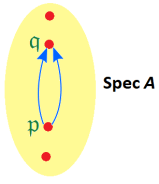
We will show how computation of Pic A leads to point addition on the elliptic curve. For each maximal ideal $\mathfrak m \subset A$ , write $[\mathfrak m]$ for its image in Pic A. Recall that points $P\in E$ correspond bijectively to maximal ideals $\mathfrak m_P \subset A$ .

Lemma 1.

Suppose $f\in A$ is not a unit. Then taking $A/(f)$ as a complex vector space, $\dim_{\mathbb C} A/(f) \le 2$ if and only if $f$ can be represented by a linear function in X, in which case

$A/(f) \cong \mathbb C[Y]/(Y^2 - \beta)$

for some $\beta\in \mathbb C$ .

Note

The intuition is that the curve $f(X, Y) = 0$ and the elliptic curve cannot have less than 3 intersection points (with multiplicity) unless we take a vertical line.

Proof

Since $Y^2 = X^3 - X$ in the ring A, without loss of generality we can write

$f(X, Y) = Y\cdot g(X) + h(X)$

for $g(X), h(X) \in \mathbb C[X]$ . The condition $\dim_{\mathbb C} A/(f) \le 2$ implies $Y^2 - X^3 + X$ and $Y\cdot g(X) + h(X)$ have at most two intersection points. Solving gives us

$g(X)^2 (X^3 - X) = h(X)^2$ .

If $g(X) \ne 0$ , the LHS has odd degree while the RHS has even degree; hence the equation has at least 3 roots and each corresponds to at least one point on the elliptic curve. If $g(X) = 0$ and $\deg h(X) = m$ , then $\dim_{\mathbb C} A/(f) = 2m$ so $h(X)$ is linear in X, and we are done. ♦

Exercise

If we replace $\mathbb C$ by a general algebraically closed field k, would the proof still work? What additional conditions (if any) need to be imposed?

Corollary 1.

No maximal ideal of A is principal.

Proof

If $\mathfrak m \subset A$ is generated by f then $A/(f) \cong \mathbb C$ , which is impossible by lemma 1. ♦

Corollary 2.

For any points $P = (\alpha_1, \beta_1)$ and $Q = (\alpha_2, \beta_2)$ on E, $\mathfrak m_P \mathfrak m_Q$ is principal if and only if

$\alpha_1 = \alpha_2, \beta_1 = -\beta_2.$

When that happens, we write $P = -Q$ .

Proof

(⇐) If $\alpha_1 = \alpha_2, \beta_1 = -\beta_2$ then setting $f = X - \alpha_1$ gives

$A/(f) \cong \mathbb C[X, Y]/(Y^2 - X^3 + X, X - \alpha_1) \cong \mathbb C[Y]/(Y^2 - (\overbrace{\alpha_1^3 - \alpha_1}^{\beta_1^2})).$

If $\beta_1 \ne 0$ , this ring has exactly two maximal ideals, corresponding to maximal ideals $\mathfrak m_P$ and $\mathfrak m_Q$ of A. If $\beta_1 = 0$ , it has exactly one maximal ideal so we still have $(f) = \mathfrak m_P^2 = \mathfrak m_P \mathfrak m_Q$ .

(⇒) If $\mathfrak m_P \mathfrak m_Q = (f)$ is principal, then $\dim_{\mathbb C} A/(f) = 2$ so by lemma 1, f can be represented by a linear function in X so we must have P and Q as described. ♦

Corollary 3.

If $P,Q\in E$ satisfy $[\mathfrak m_P] = [\mathfrak m_Q]$ , then $P=Q$ .

Proof

Let $R = -P$ as in corollary 2. Then $[\mathfrak m_P][\mathfrak m_{R}] = 1$ . By the given condition $[\mathfrak m_Q][\mathfrak m_R] = 1$ so by corollary 2 again we have $R = -Q$ and hence $P = Q$ . ♦

Lemma 2.

For any $P, Q\in E$ with $P\ne -Q$ , there is a unique $R\in E$ such that

$[\mathfrak m_P]\cdot [\mathfrak m_Q]\cdot [\mathfrak m_R] = 1.$

Proof

First suppose $P\ne \pm Q$ so P and Q have different x-coordinates. Let $f = Y - cX - d$ be the equation of PQ. We get:

$A/(f) \cong \mathbb C[X,Y]/(Y^2 - X^3 + X, Y - cX - d) \cong \mathbb C[X]/((cX+d)^2 - X^3 + X),$

which has complex dimension 3. Since $(f)$ is divisible by $\mathfrak m_P \mathfrak m_Q$ we have $(f) = \mathfrak m_P \mathfrak m_Q \mathfrak m_R$ for some $R\in E$ . Geometrically R is the third point of intersection of PQ with E, which can be equal to P or Q.

If $P = Q = (\alpha, \beta)$ with $\beta \ne 0$ , we can similarly pick a line through P of gradient $c = \frac{3\alpha^2 - 1}{2\beta}$ . Then as above $A/(f) \cong \mathbb C[X]/((cX+d)^2 - X^3 + X)$ where $(cX + d)^2 - X^3 + X$ has a double root for $X = \alpha$ (this requires some algebraic computation). Hence $(f) = \mathfrak m_P^2 \mathfrak m_R$ for some $R\in E$ . ♦

Summary.

The Picard group of A is given by

$\{ [\mathfrak m] : \mathfrak m \subset A \text{ maximal} \} \cup \{1\}$ .

In particular it is infinite.

blue-lin

Posted in Advanced Algebra | Tagged class number, dedekind domains, divisor class group, elliptic curve, minkowskis theorem, picard group | 2 Comments

Commutative Algebra 46

Posted on May 4, 2020 by limsup

Properties of Dedekind Domains

Throughout this article, A denotes a Dedekind domain.

Proposition 1.

Every fractional ideal of A can be written as

$\mathfrak m_1^{k_1} \ldots \mathfrak m_n^{k_n}, \quad k_1, \ldots, k_n \in \mathbb Z - \{0\}$

where each $\mathfrak m_i$ is a maximal ideal. The expression is unique up to permutation of terms.

Note

In particular, the maximal ideals of A generate its Picard group.

Proof

Existence. First suppose $\mathfrak a \subseteq A$ is a non-zero ideal. If $\mathfrak a = (1)$ we are done. Otherwise it is contained in some maximal ideal $\mathfrak m$ , necessarily invertible. Now $\mathfrak a \ne \mathfrak a\mathfrak m^{-1}$ , because if equality holds multiplying both sides by $\mathfrak {ma}^{-1}$ gives $\mathfrak m= A$ , so $\mathfrak a \subsetneq \mathfrak a\mathfrak m^{-1} \subseteq A$ . We replace $\mathfrak a$ by $\mathfrak a \mathfrak m^{-1}$ and repeat the process; this cannot continue indefinitely or we would have

$\mathfrak a \subsetneq \mathfrak a \mathfrak m_1^{-1}\subsetneq \mathfrak a \mathfrak m_1^{-1} \mathfrak m_2^{-1} \subsetneq \ldots$

Hence $\mathfrak a$ is a finite product of maximal ideals. Now a general fractional ideal is of the form $\frac 1 x \mathfrak a$ for a non-zero ideal $\mathfrak a \subseteq A$ and $x\in A-\{0\}$ . Write both $\mathfrak a$ and $xA$ as a product of maximal ideals and we are done.

Uniqueness. Suppose $\mathfrak m_1^{k_1} \ldots \mathfrak m_n^{k_n} = \mathfrak m_1^{j_1} \ldots \mathfrak m_n^{j_n}$ , where $j_i, k_i \in \mathbb Z$ (some possibly zero). If $(k_1, \ldots, k_n) \ne (j_1, \ldots, j_n)$ , after cancelling terms and reordering, we obtain a relation of the form:

$\mathfrak m_1^{k_1} \ldots \mathfrak m_s^{k_s} = \mathfrak m_{s+1}^{k_{s+1}} \ldots \mathfrak m_t^{k_t}, \quad k_i \in \mathbb Z_{>0}.$

This is an equality of ideals. We get a contradiction because the LHS is contained in $\mathfrak m_1$ but the RHS is not. ♦

Exercise A

Prove that an integral domain is a PID if and only if it is a Dedekind domain and a UFD. Hence we have the following Venn diagram.

venn_diagram_pid

Now we have the following.

Proposition 2.

Let M, N be non-zero fractional ideals of A. Write, as in proposition 1,

$M = \mathfrak m_1^{d_1} \mathfrak m_2^{d_2} \ldots \mathfrak m_k^{d_k}, \quad N = \mathfrak m_1^{e_1} \mathfrak m_2^{e_2} \ldots \mathfrak m_k^{e_k}$

where each $\mathfrak m_i \subset A$ is maximal and $d_i, e_i \in \mathbb Z$ . Then

$\begin{aligned} M+N &= \mathfrak m_1^{\min(d_1, e_1)} \ldots \mathfrak m_k^{\min(d_k, e_k)}\\ M\cap N &= \mathfrak m_1^{\max(d_1, e_1)} \ldots \mathfrak m_k^{\max(d_k, e_k)}\\ MN &= \mathfrak m_1^{d_1 + e_1} \ldots \mathfrak m_k^{d_k + e_k},\\ (M:N) &= \mathfrak m_1^{d_1 - e_1} \ldots \mathfrak m_k^{d_k - e_k}\end{aligned}$

Proof

Exercise. [ Localize at each $\mathfrak m_i$ ; reduce to the case where A is a dvr. ]

blue-lin

Constructing Dedekind Domains

How do we find Dedekind domains? For starters, a PID is a Dedekind domain so we have $\mathbb Z$ and $k[X]$ (for any field k), but these are not too interesting.

Here is a standard way to construct new Dedekind domains from an existing one A. Let K be its field of fractions and L be a finite extension of K; we let B be the integral closure of A in L.

dedekind_construct

Exercise B

Prove that L is the field of fractions of B.

Now B has the following properties:

it is a normal domain by construction;
dim B = 1 since B is an integral extension of A, and dim A = 1 (by main theorem here).

Hence, if we can show that B is noetherian, then it is a Dedekind domain. But this result, called the Krull-Akizuki theorem, is surprisingly hard to prove. In most cases of interest, B will turn out to be a finitely generated A-module; thus B is noetherian as an A-module and hence as a module over itself.

Examples

1. Let $K/\mathbb Q$ be a finite extension and $\mathcal O_K$ be the integral closure of $\mathbb Z$ in K. One can show that $\mathcal O_K$ is a discrete subgroup of $K$ , when we topologize $K$ by identifying it with $\mathbb Q^n$ . Hence $\mathcal O_K$ is a finitely generated $\mathbb Z$ -module; in particular it is a noetherian ring and hence a Dedekind domain. A more general result of this nature will be proven later.

2. Let k be any field such that $\mathrm{char} k \ne 2$ . The integral closure of $k[X]$ in $L = k(X)[Y]/(Y^2 - X^3 + X)$ is $A = k[X, Y]/(Y^2 - X^3 +X)$ . [ Proof: exercise. ] Since A is clearly noetherian, it is a Dedekind domain.

Exercise C

Let $m\in \mathbb Z - \{\pm 1\}$ be a square-free integer and $K = \mathbb Q(\sqrt m)$ , which is quadratic over $\mathbb Q$ . Prove that

$\mathcal O_K = \begin{cases} \mathbb Z[\frac{1 + \sqrt{m}}2], \quad &\text{if } m\equiv 1 \pmod 4, \\ \mathbb Z[\sqrt{m}], \quad &\text{if } m\equiv 2,3 \pmod 4.\end{cases}$

blue-lin

Valuation

Definition.

Let $K = \mathrm{Frac} A$ . Each maximal $\mathfrak m \subset A$ gives a function

$\nu_{\mathfrak m} : K - \{0\} \longrightarrow \mathbb Z$ ,

which takes $x$ to the exponent of $\mathfrak m$ in the above factorization of $xA$ . This is called the valuation of $x$ at $\mathfrak m$ .

Exercise D

1. Prove the following properties of $\nu = \nu_{\mathfrak m}$ : for any $x,y\in K - \{0\}$ we have:

$\nu(1) = 0, \quad \nu(xy) = \nu(x) + \nu(y), \quad \nu(x+y) \ge \min(\nu(x), \nu(y)) \text{ if } x+y\ne 0$ .

Verify that if we set $\nu(0) = \infty$ these properties hold for all $x,y\in K$ .

2. Define a distance function on K by $d(x, y) = e^{-\nu(x-y)}$ . Prove that (K, d) is a metric space, where the metric satisfies the strong triangular inequality.

$x,y, z\in K \implies d(x, z) \le \max(d(x, y), d(y, z)).$

A metric which satisfies this inequality is called an ultrametric. Interpret and prove the following statement: in an ultrametric space, every triangle is isoceles.

Valuation in Geometry

Suppose $A = \mathbb C[X, Y]/(Y^2 - X^3 + X)$ , a Dedekind domain. Recall that points P on the curve $Y^2 = X^3 - X$ correspond bijectively to maximal ideals $\mathfrak m_P \subset A$ . Then $\nu_{\mathfrak m_P}(f)$ is just the order of vanishing of f at P.

For example, let $\mathfrak m = (X, Y) = \mathfrak m_P$ where $P = (0, 0)$ ; for convenience write $\nu := \nu_{\mathfrak m}$ . Let us compute $\nu(f)$ for $f = X^2 - Y^4 \in A$ :

$X^2 - Y^4 = X^2 - (X^3 - X)^2 = 2X^4 - X^6 = X^4 ( 2 - X^2).$

Now $\nu(2 - X^2) = 0$ since f does not vanish on P. From an earlier example, we have $\mathfrak m_P^2 = (X)$ so $\nu(X) = 2$ and $\nu(X^2 - Y^4) = 8$ .

As a simple exercise, compute $\nu(Y)$ .

blue-lin

Composition Series

Recall in the last example here that for distinct maximal ideals $\mathfrak m_1, \ldots, \mathfrak m_n$ of any ring A and $k_1, \ldots, k_n \ge 1$ we have a ring isomorphism

$A/(\mathfrak m_1^{k_1} \ldots \mathfrak m_n^{k_n}) \cong A/\mathfrak m_1^{k_1} \times \ldots \times A/\mathfrak m_n^{k_n}.$

This gives the following.

Proposition 3.

If A is a Dedekind domain with finitely many maximal ideals $\mathfrak m_1, \ldots, \mathfrak m_n$ , then it is a PID.

Proof

It suffices to prove that each $\mathfrak m_i$ is principal. Let us consider $\mathfrak m_1$ . Since $\mathfrak m_i^2 \subsetneq \mathfrak m_i$ we can pick $y \in \mathfrak m_1 - \mathfrak m_1^2$ . From the isomorphism

$A/(\mathfrak m_1 \ldots\mathfrak m_n) \cong A/\mathfrak m_1 \times \ldots \times A/\mathfrak m_n$ ,

we can find $x\in A$ such that

$x\equiv y \pmod {\mathfrak m_1}, \ x \equiv 1 \pmod {\mathfrak m_2}, \ \ldots, \ x \equiv 1 \pmod {\mathfrak m_n}.$

Then x is divisible by $\mathfrak m_1$ but not its square, and not divisible by $\mathfrak m_2, \ldots, \mathfrak m_n$ . Thus $\mathfrak m_1 = (x)$ . ♦

Proposition 4.

Let $\mathfrak a \subseteq A$ be a non-zero ideal; write

$\mathfrak a = \mathfrak m_1^{k_1} \ldots \mathfrak m_n^{k_n}.$

Then the composition factors of $A/\mathfrak a$ as an A-module comprise of $k_i$ copies of $A/\mathfrak m_i$ for $1 \le i \le n$ . In particular

$l_A(A/\mathfrak a) = \sum_{i=1}^n k_i$ .

Note

Recall that the composition factors of $A/\mathfrak a$ as an A-module are identical to those as a module over itself.

Proof

The above ring isomorphism

$A/(\mathfrak m_1 \ldots\mathfrak m_n) \cong A/\mathfrak m_1 \times \ldots \times A/\mathfrak m_n$

is in fact an isomorphism of A-algebras. Hence $l_A(A/\mathfrak a) = \sum_i l_A(A/\mathfrak m_i^{n_i})$ . We obtain a series of submodules of $A/\mathfrak m^n$

$0 \subsetneq \mathfrak m^{n-1}/\mathfrak m^n \subsetneq \mathfrak m^{n-2}/\mathfrak m^n \subsetneq \ldots \subsetneq \mathfrak m/\mathfrak m^n \subsetneq A/\mathfrak m^n$

with successive quotients $\mathfrak m^i/\mathfrak m^{i+1}$ . It suffices to show each of these is of dimension 1 over $A/\mathfrak m$ . To prove that, we recall that $A_{\mathfrak m}$ is a dvr so $\mathfrak n := \mathfrak m A_{\mathfrak m}$ is a principal ideal. Since $\mathfrak m^i / \mathfrak m^{i+1}$ is already a module over $A_{\mathfrak m}$ we have:

$\dim_{A/\mathfrak m} \mathfrak m^i/\mathfrak m^{i+1} = \dim_{A_{\mathfrak m}/\mathfrak n} \mathfrak n^i / \mathfrak n^{i+1} = 1$

as desired. ♦

Note

Consider the special case where $A = k[V]$ is the coordinate ring of a variety V over an algebraically closed field k. If A is a Dedekind domain, then since $A/\mathfrak m \cong k$ for each maximal ideal $\mathfrak m \subset A$ we have

$l_A(A/\mathfrak a) = \dim_k A/\mathfrak a$ .

blue-lin

Posted in Advanced Algebra | Tagged composition factors, dedekind domains, discrete valuation rings, invertible ideals, unique factorisation, valuation | Leave a comment

Commutative Algebra 45

Posted on May 3, 2020 by limsup

Invertibility is Local

In this article, we again let A be an integral domain and K its field of fractions. We continue our discussion of invertible fractional ideals of A.

Proposition 1.

A fractional ideal M of A is invertible if and only if the following hold.

M is a finitely generated A-module.

For any maximal ideal $\mathfrak m \subset A$ , $M_{\mathfrak m}$ is an invertible fractional ideal of $A_{\mathfrak m}$ .

Proof

(⇒) This was proven earlier (propositions 2 and 5).

(⇐) It suffices to show $(A:M) M = A$ . By definition $(A:M) M\subseteq A$ . Let $\mathfrak m \subset A$ be any maximal ideal. Since M is finitely generated and $M_{\mathfrak m}$ is invertible, we have (by proposition 3 here):

$A_{\mathfrak m} = (A_{\mathfrak m} : M_{\mathfrak m})M_{\mathfrak m} = (A:M)_{\mathfrak m} M_{\mathfrak m} = [(A:M)M]_{\mathfrak m}.$

If the A-module $(A:M) M$ is contained in any maximal $\mathfrak m$ then $[(A:M)M]_{\mathfrak m} \subseteq \mathfrak m A_{\mathfrak m}$ , a contradiction. Hence $(A:M)M = A$ . ♦

Complementing the above result, we have:

Proposition 2.

Let $(A,\mathfrak m)$ be a local domain. A fractional ideal M of A is invertible if and only if it is principal and non-zero. Thus $\mathrm{Pic} A = 0$ .

Proof

Suppose M is invertible; write MN = A. Then $1 = x_1 y_1 + \ldots + x_n y_n$ for $x_i \in M$ and $y_i \in N$ . Since all $x_i y_i \in A$ and sum to 1, not all $x_i y_i$ lie in $\mathfrak m$ . Thus $x_i y_i \in A$ is invertible for some i. Multiplying $x_i$ by a unit we may assume $x_i y_i = 1$ .

It remains to show $M = Ax_i$ . Clearly since $x_i \in M$ , we have $M\supseteq A x_i$ . Conversely if $m\in M$ then $m = x_i (my_i) \in Ax_i$ since $MN\subseteq A$ . ♦

Thus we have:

Corollary 1.

A non-zero fractional ideal M of A is invertible if and only if:

it is finitely generated, and

for each maximal $\mathfrak m \subset A$ , $M_{\mathfrak m}$ is a principal fractional ideal of $A_{\mathfrak m}$ .

Example

Let $A = \mathbb Z[2\sqrt 2] = \{a + 2b\sqrt 2 : a,b \in \mathbb Z\}$ with maximal ideal $\mathfrak m = \{2a + 2b\sqrt 2: a,b\in \mathbb Z\}$ . We claim that $\mathfrak m$ is not invertible; it suffices to show that $\mathfrak m A_{\mathfrak m}$ is not a principal ideal of $A_{\mathfrak m}.$

For that we apply Nakayama’s lemma to compute $\dim_{A/\mathfrak m} \mathfrak m /\mathfrak m^2$ . Let $t = 2\sqrt 2$ ; we can check that $\mathfrak m = 2A + tA$ so $\mathfrak m^2 = 4A + 2tA = 2\mathfrak m$ since $t^2 = 8$ . Since $\mathfrak m/\mathfrak m^2$ has 4 elements, we see that $\dim_{A/\mathfrak m} \mathfrak m /\mathfrak m^2 = 2$ . Hence $\mathfrak m A_{\mathfrak m}$ is not principal.

Exercise

Let $A = \mathbb C[X, Y]/(Y^2 - X^3)$ with $\mathfrak m = (X, Y)$ . Is $\mathfrak m$ an invertible ideal?

blue-lin

Dedekind Domains

Definition.

A Dedekind domain A is an integral domain in which every fractional ideal is invertible (or equivalently, every ideal is invertible).

We obtain some immediate facts about Dedekind domains.

Since invertible ideals are finitely generated, a Dedekind domain is noetherian.
If A is a Dedekind domain so is its localization $S^{-1}A$ if $0\not\in S$ ; this follows from proposition 3 here: every ideal of $S^{-1}A$ is of the form $\mathfrak a(S^{-1}A)$ for some ideal $\mathfrak a \subseteq A$ .

Proposition 3.

In a Dedekind domain A, every non-zero prime ideal is maximal. Thus its Krull dimension is at most 1.

Hence Spec A is as follows:

one-dimensional_domains

Proof

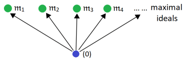
If A is a field we are done. Otherwise, we will show that every maximal ideal $\mathfrak m\subset A$ has height 1. Since $\mathfrak m$ is invertible, $\mathfrak m A_{\mathfrak m}\subset A_{\mathfrak m}$ is principal by proposition 2. By exercise A.2 here, $\mathfrak m A_{\mathfrak m}$ is a minimal non-zero prime so $\mathrm{ht} \mathfrak m = 1$ . ♦

Proposition 4.

A Dedekind domain A is normal.

Proof

Since normality is a local property, we may assume $(A, \mathfrak m)$ is local. And since $\mathfrak m$ is invertible, it is principal by proposition 2. Thus it suffices to prove the following.

If $(A,\mathfrak m)$ is a noetherian local domain such that $\mathfrak m$ is principal, then A is normal.

The whole of the next section is devoted to such rings.

blue-lin

Discrete Valuation Rings

Definition.

A discrete valuation ring (dvr) is a noetherian local domain $(A,\mathfrak m)$ such that $\mathfrak m \ne 0$ is principal. If $\mathfrak m = (\pi)$ , we call $\pi$ a uniformizer of the dvr.

Note

As we saw earlier, $(\pi)$ has height 1, so the spectrum of A is easy to describe:

spec_of_dvr

Here is an easy way to construct such rings.

Lemma.

Let A be a noetherian integral domain with a prime element $\pi \in A$ . If $\mathfrak p = (\pi)$ , then $A_{\mathfrak p}$ is a dvr.

Proof

Trivial. ♦

In particular, we can take any irreducible element π of a noetherian UFD A; then π is a prime element so $A_{(\mathfrak \pi)}$ is a dvr. Common examples include:

$\mathbb Z_{(2)} = \{\frac a b \in \mathbb Q : b \text{ odd}\},\quad k[X]_{(X)} = \{ \frac {f(X)}{g(X)} : g(0) \ne 0\},$

where k is a field.

Proposition 5.

Let A be a dvr with uniformizer $\pi$ . Then every non-zero ideal of A is uniquely of the form $(\pi^n)$ for some $n\ge 0$ .

Proof

We have $A \supsetneq (\pi) \supsetneq (\pi^2) \supsetneq \ldots$ .

First we show that $\cap_n (\pi^n) = 0$ . Indeed if $x \in \cap_n (\pi^n), x\ne 0$ then we can write $x = \pi^n u_n$ for $u_1, u_2, \ldots \in A$ . Then $u_n = \pi u_{n+1}$ for each n so $(u_1) \subsetneq (u_2) \subsetneq \ldots$ which is impossible since A is noetherian.

Now for each $x\in A-\{0\}$ , let

$\nu(x) = \max(n\ge 0 : x \in (\pi^n))$ , where $(\pi^0) = A$ .

We leave the remaining as an exercise.

Prove that $(x) = (\pi^k)$ where $k = \nu(x)$ .
Hence show that any non-zero ideal of A is of the form $(\pi^k)$ for some k. ♦

Thus a dvr is a special type of UFD with exactly one prime element (its uniformizer). This makes prime factoring in the ring rather trivial: every non-zero element is a unit times a power of the uniformizer.

Corollary 2.

A dvr is a PID, hence a UFD so it is a normal domain.

To recap, we have shown that Dedekind domains are noetherian, of Krull dimension at most 1, and normal. Next we will see that the converse is true.

blue-lin

Conditions for DVR

We have already seen:

dvr ⟹ PID ⟹ UFD ⟹ normal.

The following is a converse statement.

Proposition 6.

Let $(A,\mathfrak m)$ be a noetherian 1-dimensional local domain (i.e. A has exactly two prime ideals: 0 and $\mathfrak m$ ).

If A is normal then it is a dvr.

Proof

Pick $x\in \mathfrak m- \{0\}$ so that $A/(x)$ is a noetherian ring with exactly one prime, i.e. it is a local artinian ring, so $\mathfrak m/(x) \subset A/(x)$ is nilpotent. Thus $\mathfrak m^n \subseteq (x) \subseteq \mathfrak m$ for some n > 0. We may assume $\mathfrak m^{n-1} \not\subseteq (x)$ .

Let $\mathfrak a = \{a\in A: a\mathfrak m\subseteq (x)\}$ , an ideal of A. Fix an $a\in \mathfrak a$ and set $\alpha := \frac a x \in\mathrm{Frac} A$ . Then $\alpha \mathfrak m = \frac a x \mathfrak m \subseteq A$ is an ideal of A. If $\alpha \mathfrak m = A$ , then $\mathfrak m = \frac 1 {\alpha} A$ is principal.

Otherwise $\alpha \mathfrak m \subseteq \mathfrak m$ . We claim that $\alpha$ is integral over A. To prove this, pick a finite generating set $y_1, \ldots, y_n$ for the ideal $\mathfrak m$ ; each $\alpha y_i$ can be written as an A-linear combination of $y_1, \ldots, y_n$ so

$\alpha (y_1, \ldots, y_n)^t = M (y_1, \ldots, y_n)^t$

where M is an $n \times n$ matrix with entries in A. Hence $(\alpha I - M)(y_1, \ldots, y_n)^t = 0$ where equality holds in $\mathrm{Frac} A$ . Multiplying by the adjugate matrix, we get

$\det(\alpha I - M) \cdot (y_1, \ldots, y_n)^t = 0$ .

Since $\mathfrak m \ne 0$ , we get $\det(\alpha I - M) = 0$ ; expanding gives a monic polynomial relation in $\alpha$ with coefficients in A.

Hence $\alpha \in \mathrm{Frac} A$ is integral over A; since A is normal, $\alpha \in A$ . Thus $\frac a x \in A$ for all $a\in \mathfrak a$ so $\mathfrak a \subseteq (x)$ . Since $x \in \mathfrak a$ we have $\mathfrak a = (x)$ . But this means $\mathfrak m^{n-1} \subseteq \mathfrak a = (x)$ , a contradiction. ♦

Corollary 3.

Let A be a noetherian 1-dimensional domain. If A is normal, then it is a Dedekind domain.

Proof

Let $\mathfrak a \subseteq A$ be any ideal; it is finitely generated since A is noetherian. To prove it is invertible by proposition 1, it suffices to show $\mathfrak aA_{\mathfrak m}$ is principal for each maximal ideal $\mathfrak m$ . But $A_{\mathfrak m}$ is a local 1-dimensional noetherian domain; since it is normal, by proposition 6 it is a dvr. Hence $\mathfrak aA_{\mathfrak m}$ is principal. ♦

Summary.

Let A be an integral domain. Every non-zero ideal of A is invertible if and only if it is noetherian, normal and of Krull dimension at most 1.

If $A = k[V]$ is the coordinate ring of a variety V, geometrically the above conditions translate as follows:

Krull dimension = 1 ⟺ V is a curve;
A is a domain ⟺ V is irreducible;
A is normal ⟺ V is “smooth”.

Hence philosophically, a Dedekind domain is “like a smooth curve”.

We put the term “smooth” in quotes because we based the concept on geometric intuition rather than rigour. E.g. in our example above, the curve $Y^2 = X^3$ is not smooth at the origin.

blue-lin

Posted in Advanced Algebra | Tagged dedekind domains, discrete valuation rings, invertible ideals, local properties, localization, nakayamas lemma, normal domains | 7 Comments

Commutative Algebra 44

Posted on May 2, 2020 by limsup

Fractional Ideals

Throughout this article, let A be an integral domain and K its field of fractions. We do not assume the ring to be noetherian. The objective here is to develop the theory of multiplying and dividing certain classes of non-zero ideals so that we get a group structure.

Definition.

A fractional ideal of A is an A-submodule $M\subseteq K$ such that there is an $a\in A-\{0\}$ such that $aM\subseteq A$ .

Note

The condition $a M \subseteq A$ ensures that the elements of M do not have “too many denominators” occurring in them. Thus $\mathbb Q$ is not a fractional ideal of $\mathbb Z$ because all positive integers can appear as denominators among $a\in \mathbb Q$ .

Easy Exercise

1. Let $M\subseteq K$ be an A-submodule; prove that M is a fractional ideal if and only if there exists $a\in K - \{0\}$ such that $aM \subseteq A$ .

2. Find an example of A where K is a fractional ideal of A.

We can copy and paste many of the ideal constructions here.

Definition.

Let M, N be fractional ideals of A. We have $M\cap N, M+N$ , which are A-submodules of K. We also define the following.

$MN$ is the set of finite sums $x_1 y_1 + \ldots + x_n y_n$ , where $x_i \in M, y_i \in N$ .

$(M : N)$ is the set of all $x\in K$ such that $xN\subseteq M$ .

As before, $M\cap N$ represents the “lcm” of M and N, $M+N$ represents their “gcd”, while $MN$ , $(M : N)$ represent “product” and “division” respectively.

Be aware that unlike the case of ideals, in the definition of $(M : N)$ we have to consider all $x\in K$ .

Proposition 1.

If M and N are fractional ideals of A, so are $M \cap N$ , $M+N$ , $MN$ and; also $(M:N)$ is a fractional ideal if $N\ne 0$ .

Proof

It is easy to show they are all A-submodules of K. Now pick $a,b\in A-\{0\}$ such that $aM\subseteq A$ and $bN \subseteq A$ . Then

$\begin{aligned} ab(M+N) &= abM + abN \subseteq bA + aA \subseteq A, \\ a(M\cap N) &\subseteq aM \subseteq A, \\ ab(MN) &= (aM)(bN) \subseteq A\cdot A= A. \end{aligned}$

For the last case pick any $x\in N - \{0\}$ ; then $ax(M:N) \subseteq A$ because

$y \in (M : N) \implies yN \subseteq M \implies yx \in M \implies axy \in A.$ ♦

Exercise A

Write down and prove as many relations as you can for the above four operations. E.g.

$AM = M, \quad (M_1 + M_2)M_3 = M_1 M_3 + M_2 M_3, \quad (M_1 M_2)M_3 = M_1(M_2 M_3).$

blue-lin

Invertible Fractional Ideals

To avoid complications, henceforth we will only consider non-zero fractional ideals.

Note that the set of fractional ideals of A forms a commutative monoid under product, with identity A. In other words, it satisfies all axioms of a group except the existence of inverse. Hence we define:

Definition.

Let M be a fractional ideal of A.

We say M is principal if it is of the form $xA$ for some $x\in M$ ; we say it is invertible if MN = A for some fractional ideal N, in which case we write $N = M^{-1}$ .

An ideal of A is said to be invertible if it is invertible as a fractional ideal.

Note

Clearly principal fractional ideals are invertible. The following examples show that the converse is not true, which is why the theory is interesting.

Examples

1. Let $A = \mathbb Z[\sqrt{-5}]$ , a non-UFD. The prime ideal $\mathfrak p = (2, 1 + \sqrt{-5})$ is not principal but it is invertible because

$(2, 1 + \sqrt{-5})\cdot (2, 1-\sqrt{-5}) = (4, 2(1+\sqrt{-5}), 2(1-\sqrt{-5}), 6) = (2).$

2. Let $A = \mathbb C[X, Y]/(Y^2 - X^3 + X)$ . The maximal ideal $\mathfrak m = (X, Y) \subset A$ is invertible because

$(X, Y)^2 = (X^2, XY, Y^2) = (X^2, XY, X^3 - X) = (X).$

Proposition 2.

An invertible fractional ideal of A is finitely generated as an A-module.

Proof

Suppose $MN = A$ ; write $1 = x_1 y_1 + \ldots + x_n y_n$ for $x_i \in M, y_i \in N$ . We claim $x_1, \ldots, x_n$ generate M as an A-module. Indeed let $x\in M$ . Then

$x = 1\cdot x = (x_1 y_1 + \ldots + x_n y_n)x = x_1 (y_1 x) + \ldots + x_n (y_n x)$

and each $xy_i \in MN \in A$ . ♦

Clearly the set of invertible fractional ideals of A forms a group under product, for if M and N are invertible so is MN. The identity of this group is A. The inverse is given by the following.

Proposition 3.

Let N be an invertible fractional ideal of A. For any fractional ideal M, we have

$(M : N) = MN^{-1}$ .

Proof

We have $(MN^{-1})N = M$ and thus $MN^{-1} \subseteq (M : N)$ by definition. Conversely $(M : N)N \subseteq M$ and multiplying both sides by $N^{-1}$ gives $(M : N) \subseteq MN^{-1}$ . ♦

Note

Two special cases are important here.

Let M = A: we have $N^{-1} = (A: N) = \{x \in K : xN \subseteq A\}$ .
If M and N are invertible, so is $(M : N)$ .

Exercise

Prove that a fractional ideal is free if and only if it is principal.

Prove that in the ring $k[X, Y]/(Y^2 - X^3 + X)$ , where k is a field, the maximal ideal $\mathfrak m = (X, Y)$ is invertible. Prove also that $\mathfrak n = (X-1, Y)$ is invertible if $\mathrm{char} k \ne 2$ .

blue-lin

Picard Group

Definition.

The set of principal ideals forms a subgroup of the group of invertible fractional ideals. The resulting quotient is called the Picard group of A, i.e.

$\mathrm{Pic} A = (\text{invertible fractional ideals of } A) / (\text{principal fractional ideals of } A)$ .

Note

Every element of the Picard group can be represented by an invertible ideal $\mathfrak a \subseteq A$ .

We immediately have:

Proposition 4.

The Picard group of a UFD is trivial.

Proof

Let $\mathfrak a$ be an invertible ideal of a UFD A. By proposition 2, we can find a finite set of generators $x_1, \ldots, x_n$ of M. We claim that $x = \gcd(x_i)$ generates $\mathfrak a$ .

Since $x | x_i$ for each i we have $x_i \in xA$ and thus $\mathfrak a\subseteq xA$ .

Conversely let $y\in \mathfrak a^{-1}$ so $y\mathfrak a \subseteq A$ . For each i, $x_i y \in A$ and thus $xy = \gcd(x_i) y = \gcd(x_i y) \in A$ . So $y \in x^{-1}A$ . Thus $\mathfrak a^{-1} \subseteq x^{-1}A$ and so $xA \subseteq \mathfrak a$ . ♦

blue-lin

Localization

Now suppose $S\subseteq A$ is a multiplicative subset not including 0.

We get a map from the set of fractional ideals of A to that of $S^{-1}A$ . Indeed if $M\subseteq K$ is an A-submodule satisfying $aM\subseteq A$ then $S^{-1}M \subseteq S^{-1}K = K$ is an $(S^{-1}A)$ -submodule satisfying $\frac a 1 (S^{-1}M) \subseteq S^{-1} A$ . Clearly if M is invertible (resp. principal), so is $S^{-1}M$ .

Localization preserves the four operations we defined:

Proposition 5.

For any fractional ideals M, N of A, we have

$S^{-1}(M + N) = S^{-1}M + S^{-1}N$ ;

$S^{-1}(M \cap N) = S^{-1}M \cap S^{-1}N$ ;

$S^{-1}(MN) = (S^{-1}M)(S^{-1}N)$ ;

if $N\ne 0$ is finitely generated, then $S^{-1}(M : N) = (S^{-1}M : S^{-1}N)$ .

Note

In particular, if M is an invertible fractional ideal of A, then $S^{-1}M$ is an invertible fractional ideal of $S^{-1}A$ .

Proof

The first two properties follow from that of general submodules. The third is easy. For the last, we have

$\begin{aligned} &S^{-1}(M:N) S^{-1}N = S^{-1}((M : N)N) \subseteq S^{-1}M \\ \implies &S^{-1}(M:N) \subseteq (S^{-1}M : S^{-1}N).\end{aligned}$

For the reverse inclusion suppose $\frac y s S^{-1}N \subseteq S^{-1}M$ for $\frac y s \in S^{-1}A-\{0\}$ . Write $N = Ax_1 + \ldots + Ax_n$ ; then $\frac{yx_i} 1 \in S^{-1}M$ for each i. Write $\frac {yx_i} 1 = \frac {z_i}{s_i}$ for $z_i \in M$ and $s_i \in S$ ; we see that $tyx_i \in M$ for each i where $t = s_1 \ldots s_n$ . [ Recall that A is an integral domain. ] Hence

$tyN\subseteq M \implies ty \in (M : N)\implies \frac y s \in S^{-1}(M:N)$ . ♦

Corollary 1.

We obtain a group homomorphism

$\mathrm{Pic} A \longrightarrow \mathrm{Pic} S^{-1}A,\quad [M] \mapsto [S^{-1}M].$

where M is an invertible ideal of A representing an element of $\mathrm{Pic} A$ .

Example

Let $A = \mathbb Z[\sqrt{-5}]$ with $\mathfrak p =(2, 1 + \sqrt{-5}) \subset A$ , a non-principal invertible ideal. If $S = \{2^n\}$ then $\mathrm{Pic} A \to \mathrm{Pic} S^{-1}A$ takes $\mathfrak p \mapsto 1$ since $\mathfrak p \cdot S^{-1}A$ is generated by $(1 + \sqrt{-5})$ .

blue-lin

Posted in Advanced Algebra | Tagged fractional ideals, ideal division, invertible ideals, localization, picard group, principal ideals | 5 Comments

Commutative Algebra 43

Posted on May 1, 2020 by limsup

Catenary Rings

Let us look at prime chains in greater detail.

Definition.

Let $\mathfrak p_0 \subsetneq \ldots \subsetneq \mathfrak p_d$ be a chain of prime ideals of a ring A. We say the chain is

saturated if for any prime ideal $\mathfrak q$ of A,

$\mathfrak p_i \subseteq \mathfrak q \subseteq \mathfrak p_{i+1} \implies \mathfrak q = \mathfrak p_i \text{ or } \mathfrak q = \mathfrak p_{i+1}$ ;

maximal if it is saturated, $\mathfrak p_0$ is a minimal prime and $\mathfrak p_d$ is a maximal ideal.

In words, saturated means we cannot insert a prime ideal between any two consecutive terms of a chain; maximal means in addition, we cannot extend the chain further in either direction.

Definition.

A ring is said to be catenary if, for all primes $\mathfrak p, \mathfrak q \subset A$ , all saturated prime chains with fixed ends

$\mathfrak p = \mathfrak p_0 \subsetneq \mathfrak p_1 \subsetneq \ldots \subsetneq \mathfrak p_d = \mathfrak q$

have the same length d.

catenary_spec

Note

If A is a catenary ring, so is any of its quotient $A/\mathfrak a$ or localization $S^{-1}A$ since the resulting spectrum is a subspace of Spec A.

blue-lin

Clarifications

Since dimension theory can be rather tricky, we will spend some time to clarify some of the above concepts.

1. On Catenary Rings

Catenary rings A are extremely common. In fact, it takes quite a bit of effort to construct a noetherian ring which is not catenary and such examples are usually pathological. See this article from Stacks project for an explicit construction by Nagata.

2. Maximal Prime Chains in Catenary Rings

warning However, even in a catenary ring A, not all maximal prime chains may be of the same length. The reason is rather simple: A can have multiple minimal prime ideals and multiple maximal ideals. The catenary condition does not specify that every saturated prime chain from every minimal prime to every maximal prime must be of the same length.

E.g. in the following Spec A, the blue prime chains may be longer than the green ones.

catenary_spec_v2

With multiple minimal primes, it is easy to construct catenary rings with maximal prime chains of different lengths. For example if $B = A_1 \times A_2$ , the set of prime chains of B is the union of that of $A_1$ and of $A_2$ . So if we pick $A_1, A_2$ of different dimensions like $B = \mathbb C \times \mathbb C[X]$ we get maximal prime chains of different lengths:

$0 \times \mathbb C[X], \qquad \mathbb C \times 0 \subset \mathbb C \times \mathbb (X)$ .

3. Catenary Rings Which Are Integral Domains

What if we specify that A is an integral domain? This ensures that there is a unique minimal prime: 0 itself. There remains the possibility of multiple maximal ideals. When A is a finitely generated algebra over a field, indeed all maximal prime chains have the same length (to be proven later).

In the general case, we have the following counter-example $A = \mathbb Z_{\mathfrak p}[X]$ where $\mathfrak p = 2\mathbb Z$ . This has maximal prime chains

$0 \subset (2X - 1), \qquad 0 \subset (2) \subset (2, X)$

of different lengths.

4. Dimension of Noetherian Rings

If A is a noetherian ring, every chain of ideals of A must eventually terminate so we cannot have infinite prime chains. But this does not mean $\dim A$ must be finite, for A may have maximal prime chains of arbitrary length. For example, Nagata constructed a noetherian ring A whose spectrum looks like the following,

nagata_infinite_dim

where the i-th column is a maximal prime chain of length i-1. In particular, $dim A = \infty$ .

Exercise A

1. Decide if each of the following is true or false.

If A is a catenary ring which is a local integral domain, then all maximal prime chains have the same length.
If A is a catenary ring which is a local ring, then all maximal prime chains have the same length.

2. Let A be a noetherian domain.

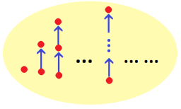
Prove that if the prime ideal $\mathfrak p \ne 0$ of A is principal, then it is a minimal non-zero prime.
Prove that if A is a UFD, any minimal non-zero prime ideal is principal.

3. Prove that the two prime chains in example 3 are maximal.

4. Prove that any maximal prime chain of $\mathbb Z[X]$ has length 2. In particular, $\mathbb Z[X]$ is catenary and hence the ring in example 3 is catenary since it is a localization of $\mathbb Z[X]$ .

blue-lin

More Consequences of NNT

Now we consider finitely generated k-algebras where k is a field.

Proposition 1.

Let $A = k[X_1, \ldots, X_n]$ . All maximal prime chains of A have the same length n.

Note

Although we already have dim A = n, this is a significantly stronger result.

Proof

The proof is by induction on n. We may assume $n\ge 1$ .

Note that 0 is a prime ideal of A. Let $\mathfrak p$ be a minimal non-zero prime and $B = A/\mathfrak p$ . By exercise A.2 above $\mathfrak p =(f)$ since A is a UFD. By exercise B here, B has transcendence degree n – 1 so by induction hypothesis any maximal prime chain of B has length n – 1. Since $\mathfrak p$ is an arbitrary minimal non-zero prime this shows that any maximal prime chain of A has length n. ♦

With this as a base, we may now prove the more general result.

Proposition 2.

Let A be a finitely generated k-algebra which is also an integral domain. All maximal prime chains of A have the same length n.

Note

We must have $n = \dim A = \mathrm{trdeg} A/k$ .

Proof

Since A is finitely generated we can write it as $A\cong k[X_1, \ldots, X_m]/\mathfrak p$ for a prime ideal $\mathfrak p \subset k[X_1, \ldots, X_m]$ . Fix a saturated prime chain of $k[X_1, \ldots, X_m]$ which starts at 0 and ends at $\mathfrak p$ ; let j be its length.

Now suppose we pick any maximal prime chain of A; let l be its length. The chain must start at 0 and end at a maximal ideal, which corresponds to a prime chain of $k[X_1, \ldots, X_m]$ starting at $\mathfrak p$ and ending at a maximal ideal (containing $\mathfrak p$ ). Appending the prior chain, we thus obtain a maximal prime chain of $k[X_1, \ldots, X_m]$ . By proposition 1, we must have $j + l = m$ so $l = m-j$ is independent of the maximal prime chain of A we chose. ♦

blue-lin

Height of an Ideal

Definition.

Let $\mathfrak p \subset A$ be a prime ideal. The height of $\mathfrak p$ , denoted by $\mathrm{ht} \mathfrak p$ , is the supremum of the lengths of prime chains ending at $\mathfrak p$ .

In other words $\mathrm{ht} \mathfrak p = \dim A_{\mathfrak p}$ . Since $\dim A/\mathfrak p$ is the supremum of the lengths of prime chains starting from $\mathfrak p$ , it follows that we always have

$\mathrm{ht} \mathfrak p + \dim A/\mathfrak p \le \dim A.$

We can also define the height of any ideal.

Definition.

Let $\mathfrak a\subseteq A$ be an ideal. The height of $\mathfrak a$ , denoted by $\mathrm{ht}\mathfrak a$ , is the infimum of $\mathrm{ht} \mathfrak p$ over all primes $\mathfrak p \supseteq \mathfrak a$ .

Note

Here is the intuition behind the definition. Note that $\dim A/\mathfrak a$ is the supremum of $\dim A/\mathfrak p$ over all $\mathfrak p \supseteq \mathfrak a$ . Thus to “compensate” for taking the supremum here, we let $\mathrm{ht} \mathfrak a$ take the infimum of $\mathrm{ht}\mathfrak p$ over all $\mathfrak p\supseteq \mathfrak a$ .

From the previous section, we obtain:

Corollary 1.

If A is a finitely generated k-algebra and also an integral domain, then for any prime ideal $\mathfrak p\subset A$ we have

$\mathrm{ht} \mathfrak p + \dim A/\mathfrak p = \dim A.$

In particular, A is a catenary ring.

More generally we have:

Corollary 2.

Any finitely generated algebra A over a field is catenary.

Hence so is any localization of such an algebra.

Proof

A must be a quotient of some $k[X_1, \ldots, X_m]$ so it is catenary. ♦

blue-lin

Posted in Advanced Algebra | Tagged algebras, catenary rings, krull dimension, noether normalization, noetherian | 2 Comments

Commutative Algebra 42

Posted on April 30, 2020 by limsup

Noether Normalization Theorem

Throughout this article, k is a field, not necessarily algebraically closed.

Definition.

Let A be a finitely generated k-algebra which is an integral domain.

We say $\alpha_1, \ldots, \alpha_n \in A$ are algebraically independent over k if they are so as elements of $\mathrm{Frac} A$ .

The transcendence degree of A over k refers to that of $\mathrm{Frac} A$ over k.

Immediately we present the main theorem of the day.

Noether Normalization Theorem (NNT).

Let $A$ be a finitely generated k-algebra. There exist $\alpha_1, \ldots, \alpha_n \in A$ which are algebraically independent over k such that A is finite over $k[\alpha_1, \ldots, \alpha_n]$ .

Note

Hence Frac(A) is algebraic over $k(\alpha_1, \ldots, \alpha_n)$ so $\mathrm{trdeg} A/k = n$ .

Proof

Write $A = k[x_1, \ldots, x_m]$ for some $x_1, \ldots, x_m \in A$ . We will prove the result by induction on m; when m = 0 there is nothing to show so suppose m ≥ 1.

Let $B:=k[x_1, \ldots, x_{m-1}]$ so that $k\subseteq B \subseteq A$ . By induction hypothesis we can find $\alpha_1, \ldots, \alpha_n \in B$ which are algebraically independent over k and B is finite over $k[\alpha_1, \ldots, \alpha_n]$ . Now we consider whether $x := x_m$ is algebraic or transcendental over Frac(B).

Case 1 : $x_m$ is transcendental over Frac(B).

Thus $\alpha_1, \ldots, \alpha_n, x_m$ are algebraically independent over k. Also

$k[\alpha_1, \ldots, \alpha_n, x_m] \subseteq B[x_m] = A$

is a finite extension so we are done.

Case 2 : $x_m$ is algebraic over Frac(B).

Since $x_m$ is algebraic over $k(\alpha_1, \ldots, \alpha_n)$ we can write

$x_m^d + c_{d-1} x_m^{d-1} + \ldots + c_1 x_m + c_0 = 0$ for some $c_0, \ldots, c_{d-1} \in k(\alpha_1, \ldots, \alpha_n)$ .

Clearing denominators we get

$p_d(\alpha_1, \ldots, \alpha_n) x_m^d + p_{d-1}(\alpha_1, \ldots, \alpha_n) x_m^{d-1} + \ldots + p_0(\alpha_1, \ldots, \alpha_n) = 0$

where $p_i \in k[X_1, \ldots, X_n]$ , not all zero. We reparametrize $\beta_i = \alpha_i - x_m^{d_i}$ for $1\le i\le n$ , where the $d_i \ge 0$ will be determined later. Substituting then gives us

$\sum_{j=0}^d p_j(\beta_1 + x_m^{d_1}, \beta_2 + x_m^{d_2}, \ldots, \beta_n + x_m^{d_n}) x_m^j = 0.$

Claim.

There exist $d_1, \ldots, d_n \ge 0$ such that expanding the above gives

$\sum_{j=0}^D q_j(\beta_1, \ldots, \beta_n) x_m^j = 0$ where $q_j \in k[X_1, \ldots, X_n]$ and $q_D \in k-\{0\}$ .

Proof of Claim.

Pick $M > \max(d, \deg p_0, \ldots, \deg p_d)$ and let $d_i = M^i$ . Expanding $p_j(\beta_1 + x_m^{d_1}, \beta_2 + x_m^{d_2}, \ldots, \beta_n + x_m^{d_n}) x_m^j$ , we obtain a sum of terms of the form

$(\beta_1 + x_m^{d_1})^{e_1} (\beta_2 + x_m^{d_2})^{e_2} \ldots (\beta_n + x_m^{d_n})^{e_n}\cdot x_m^j, \quad e_1, \ldots, e_n \ge 0.$

The top exponent of $x_m$ upon expansion is $d_1 e_1 + \ldots + d_n e_n + j = M e_1 + \ldots + M^n e_n + j$ . Since $0\le e_1, \ldots, e_n, j < M$ , we see that these values are distinct across all the terms. Thus there is a unique term of $x_m^D$ where D is the maximum over these $j + \sum_i d_i e_i$ .

This proves the claim. ♦

Resuming the proof of the theorem, we see that $x_m$ is integral over $k[\beta_1, \ldots, \beta_n]$ , so we have finite extensions

$k[\beta_1, \ldots, \beta_n] \subseteq k[\beta_1, \ldots, \beta_n, x_m] = k[\alpha_1, \ldots, \alpha_n, x_m] \subseteq B[x_m] = A$

and we are done. ♦

Exercise

Let $k = \mathbb C$ . For each of the following A, find an algebraically independent sequence $\alpha_1, \ldots, \alpha_n \in A$ such that $\mathbb C[\alpha_1, \ldots, \alpha_n] \subseteq A$ is finite.

$\mathbb C[X, Y]/(XY - 1), \quad \mathbb C[X, Y, Z]/(XY + YZ + ZX - 1).$

blue-lin

Proof of Nullstellensatz

The NNT allows us to prove the Nullstellensatz quite easily.

Corollary 1.

Let A be a finitely generated k-algebra. If A is a field, then it is a finite extension of k.

Proof

By NNT we can find algebraically independent $\alpha_1, \ldots, \alpha_n \in A$ over k such that $k[\alpha_1, \ldots, \alpha_n] \subseteq A$ is finite. If $n\ge 1$ then $\frac 1 {\alpha_1} \in A$ is integral over $k[\alpha_1, \ldots, \alpha_n]$ which is absurd since $k[\alpha_1, \ldots, \alpha_n]$ is a UFD and hence normal. ♦

For the rest of this section suppose k is algebraically closed. Recall the correspondence between radical ideals of $A := k[X_1, \ldots, X_n]$ and closed subsets $V\subseteq \mathbb A^n(k)$ .

Corollary 2.

If $\mathrm a \subseteq A$ is a proper ideal then $V(\mathfrak a) \ne\emptyset$ .

Proof

Let $\mathfrak m$ be any maximal ideal of A containing $\mathfrak a$ . Then $A/\mathfrak m$ is a finitely generated k-algebra so by corollary 1, it is isomorphic to k as a k-algebra. From $A/\mathfrak m \cong k$ , suppose $X_i \mapsto v_i \in k$ . Then $\mathfrak m = (X_1 - v_1, \ldots, X_n - v_n)$ . Hence $(v_1, \ldots, v_n) \in V(\mathfrak a)$ . ♦

Theorem (Nullstellensatz).

If $\mathfrak a \subseteq A$ is a radical ideal, then

$IV(\mathfrak a) = \mathfrak a$ .

Proof

We already know (⊇) holds. For (⊆), pick any $f\in IV(\mathfrak a)$ . Since A is noetherian $\mathfrak a$ has a finite set of generators $(f_1, \ldots, f_k)$ . Consider the ideal $\mathfrak b := (f_1, \ldots, f_k, Y\cdot f - 1)$ of $B = k[X_1, \ldots, X_n, Y]$ . Note that $B/\mathfrak b \cong (A/\mathfrak a)_f$ . We claim that $\mathfrak b = B$ .

If not, by corollary 2 there exists a point $(v_1, \ldots, v_n, w) \in \mathbb A^{n+1}$ such that $f_i (v_1, \ldots, v_n) = 0$ for $1\le i\le k$ and $f(v_1, \ldots, v_n)w = 1$ . Then $(v_1, \ldots, v_n) \in V(\mathfrak a)$ but $f(v_1,\ldots, v_n) \ne 0$ , contradicting $f\in IV(\mathfrak a)$ .

Hence $(A/\mathfrak a)_f = 0$ so $f^m \in \mathfrak a$ for some m > 0. Since $\mathfrak a$ is radical this means $f\in \mathfrak a$ . ♦

blue-lin

Consequences of NNT

This gives us the following highly non-trivial result.

Proposition 1.

For any field k, $\dim k[X_1, \ldots, X_n] = n$ .

Proof

(≥) Take the prime chain $0 \subset (X_1) \subset (X_1, X_2) \subset \ldots \subset (X_1, \ldots, X_n)$ .

(≤) The proof is by induction on n : when n = 0 this is clear so let n > 0. Suppose $\mathfrak p \subset k[X_1, \ldots, X_n]$ is any non-zero prime ideal. Now $\mathfrak p$ contains some irreducible f so for $A = k[X_1, \ldots, X_n]/\mathfrak p$ , by exercise B here, we have

$\mathrm{trdeg} A/k \le n-1.$

By NNT, we can find $\alpha_1, \ldots, \alpha_m \in A$ which are algebraically independent such that A is finite over $k[\alpha_1, \ldots, \alpha_m]$ where $m = \mathrm{trdeg} A/k \le n-1$ . By induction hypothesis,

$\dim k[\alpha_1, \ldots, \alpha_m] = m$

and since A is finite over it we have $\dim A = m \le n-1$ too. Since $\dim A/\mathfrak p \le n-1$ for all non-zero prime $\mathfrak p$ we have $\dim A \le n$ . ♦

Corollary 3.

Let A be a finitely generated k-algebra which is also an integral domain. Then

$\dim A = \mathrm{trdeg} A/k$ .

Proof

By NNT pick $\alpha_1, \ldots, \alpha_n \in A$ which are algebraically independent over k such that $k[\alpha_1, \ldots, \alpha_n] \subseteq A$ is finite. Then

$\dim A = \dim k[\alpha_1, \ldots, \alpha_n] = n.$ ♦

Next, the following is consistent with our intuition.

Proposition 2.

Now suppose k is algebraically closed.

If A, B are finitely generated k-algebras which are integral domains, then

$\dim (A\otimes_k B) = \dim A + \dim B.$

Note

Recall (exercise B here) that if we write $A\cong k[V]$ and $B \cong k[W]$ for irreducible affine varieties, then $A\otimes_k B \cong k[V\times W]$ is an integral domain since $V\times W$ is also irreducible.

Proof

Pick $\alpha_1, \ldots, \alpha_n \in A$ (resp. $\beta_1, \ldots, \beta_m \in B$ ) which are algebraically independent over k such that

$k[\alpha_1, \ldots, \alpha_n] \subseteq A, \quad k[\beta_1, \ldots, \beta_m] \subseteq B$

are finite extensions. Now we have an injection

$k[X_1, \ldots, X_n, Y_1, \ldots, Y_m] \cong k[\alpha_1, \ldots, \alpha_n] \otimes_k k[\beta_1, \ldots, \beta_m] \hookrightarrow A\otimes_k B$

which is also a finite extension. Thus $\dim (A\otimes_k B) = m + n$ . ♦

blue-lin

Posted in Advanced Algebra | Tagged finite extensions, integral extensions, krull dimension, noether normalization, nullstellensatz, transcendence degree | 4 Comments

Commutative Algebra 41

Posted on April 29, 2020 by limsup

Basic Definitions

The objective of this article is to establish the theory of transcendence bases for field extensions. Readers who are already familiar with this may skip the article. We will focus on field extensions $K\subseteq L$ here.

Definition.

Let $K\subseteq L$ be a field extension. Elements $\alpha_1, \ldots, \alpha_n \in L$ are said to be algebraically dependent over K if

$\exists p \in K[X_1, \ldots, X_n] - \{0\}, \ p(\alpha_1, \ldots, \alpha_n) = 0.$

Otherwise, $\alpha_1, \ldots, \alpha_n$ are algebraically independent over K.

We say $(\alpha_1, \ldots, \alpha_n)$ forms a transcendence basis of L over K if it is algebraically independent over K and L is algebraic over $K(\alpha_1, \ldots, \alpha_n)$ .

If such a basis exists for $K\subseteq L$ , we say L has finite transcendence degree over K, and write

$n = \mathrm{trdeg} L/K$ ,

the transcendence degree of L over K.

Exercise A

Prove that if $A = \mathbb C[X, Y]/(Y^2 - X^3 + X)$ then $L := \mathrm{Frac} A \cong \mathbb C(X)[Y]/(Y^2 - X^3 + X)$ so $\alpha_1 = X$ forms a transcendentce basis of L over $\mathbb C$ .

Note that a priori, it is not clear that the transcendence basis is well-defined: could we perhaps choose two transcendence bases of different sizes? The answer is no as we will see.

Lemma 1.

For $\alpha_1, \ldots, \alpha_n \in L$ write $L' = K(\alpha_1, \ldots, \alpha_n)$ for the field extension of K generated by $\alpha_1, \ldots, \alpha_n$ .

If $\alpha_1, \ldots, \alpha_n$ are algebraically independent over K, then every element of L’ can be uniquely written as $f(\alpha_1, \ldots, \alpha_n)$ as $f$ runs through all rational functions $K(X_1, \ldots, X_n)$ . Thus we have an isomorphism:

$K(X_1, \ldots, X_n) \cong L' = K(\alpha_1, \ldots, \alpha_n), \quad X_i \mapsto \alpha_i$ .

Proof

Consider the K-algebra homomorphism $K[X_1, \ldots, X_n] \to L$ which takes $X_i \mapsto \alpha_i$ for each $1\le i \le n$ . By definition of algebraic independence this map is injective so we get an embedding

$K(X_1, \ldots, X_n) = \mathrm{Frac}(K[X_1, \ldots, X_n]) \longrightarrow L$

of fields, whose image is clearly L’. ♦

blue-lin

Swapping Lemma

The following will be repeatedly used throughout the article.

Key Observation.

Let $K\subseteq L$ be a field extension and $\alpha_1, \ldots, \alpha_n\in L$ be algebraically independent over K. Let $\beta \in L$ .

Then $\alpha_1, \ldots, \alpha_n, \beta$ are algebraically dependent over K if and only if $\beta$ is algebraic over $K(\alpha_1, \ldots, \alpha_n)$ .

Note

Compare this with the linear algebra variant: if V is a vector space and $v_1, \ldots, v_n \in V$ are linearly independent, then for $w\in V$ , $v_1, \ldots, v_n, w$ are linearly dependent if and only if w is a linear combination of $v_1, \ldots, v_n$ .

Proof

(⇒) If $\alpha_1, \ldots, \alpha_n, \beta$ are algebraically dependent over K we have a non-zero polynomial $p \in K[X_1, \ldots, X_n, Y]$ such that $p(\alpha_1, \ldots, \alpha_n, \beta) = 0$ . This polynomial must involve Y or we would obtain a polynomial relation in $\alpha_1, \ldots, \alpha_n$ , a contradiction. Taking

$q(Y) := p(\alpha_1, \ldots, \alpha_n, Y) \in K(\alpha_1, \ldots, \alpha_n)[Y] \cong K(X_1, \ldots, X_n)[Y]$ ,

we see that $q \ne 0$ and $q(\beta) = 0$ . ♦

(⇐) If $\beta$ is algebraic over $K' := K(\alpha_1, \ldots, \alpha_n)$ pick $c_0, \ldots, c_d \in K'$ , not all zero, such that

$c_d \beta^d + c_{d-1} \beta^{d-1} + \ldots + c_1 \beta + c_0 = 0.$

Clearing denominators, we assume each $c_i \in K[\alpha_1, \ldots, \alpha_n]$ so $p(\alpha_1, \ldots, \alpha_n, \beta) = 0$ for some non-zero polynomial $p(X_1, \ldots, X_n, Y)$ with coefficients in K. ♦

Here is the main result.

Swapping Lemma.

Let $\alpha_1, \ldots, \alpha_n$ be a transcendence basis of L over K and $\beta \in L$ be transcendental (i.e. not algebraic) over K. Then there exists an $\alpha_i$ such that

$\alpha_1, \ldots, \alpha_{i-1}, \beta, \alpha_{i+1}, \ldots \alpha_n$

form a transcendence basis of L over K.

Furthermore if $\beta, \alpha_1, \ldots, \alpha_j$ are algebraically independent over K, then we can pick $\alpha_i$ from $\alpha_{j+1}, \ldots, \alpha_n$ .

swapping_lemma

Proof

By assumption $\beta$ is algebraic over $K(\alpha_1, \ldots, \alpha_n)$ . Thus by the key observation, $\alpha_1, \ldots, \alpha_n, \beta$ are algebraically dependent. Assume

$\beta, \alpha_1, \ldots, \alpha_j$ are algebraically independent but
$\beta, \alpha_1, \ldots, \alpha_{j+1}$ are algebraically dependent.

We claim that swapping $\alpha_{j+1}$ with $\beta$ also gives a transcendence basis.

Indeed let $K' = K(\alpha_1, \ldots, \alpha_j, \beta, \alpha_{j+2}, \ldots, \alpha_n)$ . By the key observation, $\alpha_{j+1}$ is algebraic over $K(\beta, \alpha_1, \ldots, \alpha_j)$ and hence over K’. So we have algebraic extensions $K' \subseteq K'(\alpha_{j+1}) \subseteq L$ .

It remains to show that $\alpha_1, \ldots, \alpha_j, \alpha_{j+2}, \ldots, \alpha_n, \beta$ are algebraically independent. If not, by the key observation $\beta$ is algebraic over $K'' := K(\alpha_1, \ldots, \alpha_j, \alpha_{j+2}, \ldots, \alpha_n)$ and we have algebraic extensions $K'' \subseteq K''(\beta) = K' \subseteq K'(\alpha_{j+1})$ , so $\alpha_{j+1}$ is algebraic over $K''$ , a contradiction. ♦

blue-lin

Transcendence Degree is Well-Defined

Proposition 1.

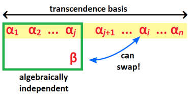
If $\alpha_1, \ldots, \alpha_n$ is a transcendence basis for $L/K$ and $\beta_1, \ldots, \beta_m \in L$ are algebraically independent over K, then

$m\le n$ and

we can replace m terms of $\alpha_1, \ldots, \alpha_n$ by $\beta_1, \ldots, \beta_m$ to obtain another transcendence basis for L over K.

Proof

We repeatedly apply swapping lemma. If m = 0, there is nothing to prove; otherwise by swapping lemma, we can swap out some element of $\alpha_1, \ldots, \alpha_n$ with $\beta_1$ to obtain another transcendence basis.

At each stage, suppose we have a transcendence basis $\beta_1, \ldots, \beta_j$ together with n–j elements of $\alpha_i$ . If j = m we are done. If j = n then $\beta_1, \ldots, \beta_j$ is already a transcendence basis so we also have j = m. Hence suppose $j<n$ and $j<m$ .

Since $\beta_1, \ldots, \beta_j, \beta_{j+1}$ are algebraically independent, swapping lemma asserts we can swap out another $\alpha_i$ with $\beta_{j+1}$ so we get a transcendence basis $\beta_1, \ldots, \beta_{j+1}$ together with n–j-1 elements of $\alpha_i$ . Eventually, we obtain a transcendence basis comprising of $\beta_1,\ldots, \beta_m$ with n – m elements of $\alpha_i$ . ♦

Corollary 1.

Any two transcendence bases of L/K have cardinality n so $\mathrm{trdeg} L/K$ is well-defined.

Proof

For any transcendence bases $\alpha_1, \ldots, \alpha_n$ and $\beta_1, \ldots, \beta_m$ , proposition 1 says $m\le n$ and $n\le m$ . ♦

blue-lin

Transitivity

Lemma 2.

Let $K\subseteq L$ be a field extension and $\alpha_1, \ldots, \alpha_m \in L$ such that L is algebraic over $K(\alpha_1, \ldots, \alpha_m)$ .

Then $(\alpha_1, \ldots, \alpha_m)$ contains a transcendence basis of L over K.

Proof

Pick a maximal algebraically independent subset of $(\alpha_1, \ldots, \alpha_m)$ . Upon reordering suppose this is $(\alpha_1, \ldots, \alpha_n)$ ; set $K' := K(\alpha_1, \ldots, \alpha_n)$ . By maximality of $(\alpha_1, \ldots, \alpha_n)$ , each of $\alpha_{n+1}, \ldots, \alpha_m$ is algebraic over $K'$ . Hence we get algebraic extensions

$K' \subseteq K'(\alpha_{n+1}, \ldots, \alpha_m) = K(\alpha_1, \ldots, \alpha_m) \subseteq L$

and we are done. ♦

Proposition 2.

Let $K\subseteq L \subseteq M$ be field extensions. Then M has finite transcendence degree over K if and only if M has finite transcendence degree over L and L has finite transcendence degree over K, in which case

$\mathrm{trdeg} M/K = \mathrm{trdeg} M/L + \mathrm{trdeg} L/K.$

Proof

(⇒) Let $\alpha_1, \ldots, \alpha_n$ be a transcendence basis of M over K. In particular M is algebraic over $L(\alpha_1, \ldots, \alpha_n)$ so by lemma 2, there exists a subset of $\alpha_1, \ldots, \alpha_n$ which forms a transcendence basis of M over L.

Next suppose $\beta_1, \ldots, \beta_m \in L$ are algebraically independent over K. By proposition 1, $m\le n$ so there exists a maximal algebraically independent sequence $\beta_1, \ldots, \beta_m$ for L/K. By key observation it follows that any $\beta \in L$ is algebraic over $K(\beta_1, \ldots, \beta_m)$ .

(⇐) Pick transcendence bases $\alpha_1, \ldots, \alpha_n$ for L over K, and $\beta_1, \ldots, \beta_m$ for M over L. We claim that $\alpha_1, \ldots, \alpha_n, \beta_1, \ldots, \beta_m$ form a transcendence basis of M over K, which would complete the proof.

Suppose $p(\alpha_1, \ldots, \alpha_n, \beta_1, \ldots, \beta_m) = 0$ for a non-zero $p\in K[X_1, \ldots, X_n, Y_1, \ldots, Y_m]$ . Then $q(\alpha_1, \ldots, \alpha_n, Y_1, \ldots, Y_m) \in L[Y_1, \ldots, Y_m]$ is a polynomial relation for $\beta_i$ ; since these are algebraically independent we have $q=0$ . But the coefficients of q are polynomials in $\alpha_j$ ; since $\alpha_j$ are algebraically independent, we also get $p=0$ .

Finally, since $K(\alpha_1, \ldots, \alpha_n) \subseteq L$ is algebraic, so is

$K(\alpha_1, \ldots, \alpha_n, \beta_1, \ldots, \beta_m) \subseteq L(\beta_1, \ldots, \beta_m)$

since the RHS is generated as a field by L and $\beta_1, \ldots, \beta_m$ , all algebraic over the LHS. Furthermore, $L(\beta_1, \ldots, \beta_m) \subseteq M$ is algebraic by assumption. Thus

$K(\alpha_1, \ldots, \alpha_n, \beta_1, \ldots, \beta_m) \subseteq M$

is an algebraic extension as desired. ♦

Exercise B

Let $A = K[X_1, \ldots, X_n]/(f)$ where $f\in K[X_1, \ldots, X_n]$ is irreducible. Prove that $\mathrm{Frac} A$ has transcendence degree n – 1 over K.

blue-lin

Posted in Advanced Algebra | Tagged algebraic extensions, fields, transcendence basis, transcendence degree | 2 Comments

Commutative Algebra 40

Posted on April 28, 2020 by limsup

More on Integrality

Lemma 1.

Let $A\subseteq B$ be an integral extension. If $\mathfrak b \subseteq B$ is an ideal and $\mathfrak a = \mathfrak b \cap A$ , the resulting injection $A/\mathfrak a \hookrightarrow B/\mathfrak b$ is an integral extension.

Proof

Any element of $B/\mathfrak b$ can be written as $x + \mathfrak b$ , $x\in B$ . Then x satisfies a monic polynomial relation:

$x^n + a_{n-1} x^{n-1} + \ldots + a_1 x + a_0 = 0, \quad a_0, \ldots, a_{n-1} \in A$ .

Taking the relation modulo $\mathfrak b$ gives a monic polynomial relation for $x + \mathfrak b$ with coefficients in $A/\mathfrak a$ . ♦

Lemma 2.

Let $A\subseteq B$ be an integral extension and suppose C is the integral closure of A in B. If $S \subseteq A$ is a multiplicative subset, then $S^{-1}C$ is the integral closure of $S^{-1}A$ in $S^{-1}B$ .

Proof

Suppose $\frac x s \in S^{-1}C$ where $x\in C$ and $s\in S$ . Since x is integral over A we have $x^n + a_{n-1} x^{n-1} + \ldots + a_0 = 0$ for some $a_i \in A$ . Then in $S^{-1}C$ we have the equality

$(\frac x s)^n + \frac{a_{n-1}}s (\frac x s)^{n-1} + \ldots + \frac{a_0}{s^n} = 0, \quad \frac {a_i}{s^{n-i}} \in S^{-1}A$

so $\frac x s$ is integral over $S^{-1}A$ .

Conversely, suppose $\frac x s\in S^{-1}B$ is integral over $S^{-1}A$ where $x\in B$ and $s\in S$ . Then $\frac x 1\in S^{-1}B$ is also integral over $S^{-1}A$ so

$(\frac x 1)^n + \frac {a_{n-1}}{s_{n-1}} (\frac x 1)^{n-1} + \ldots + \frac{a_1}{s_1} (\frac x 1) + \frac{a_0}{s_0} = 0$ for some $\frac{a_i}{s_i} \in S^{-1}A.$

Multiplying by $s_0 \ldots s_{n-1}$ , there exist $t\in S$ and $a_0', \ldots, a_{n-1}' \in A$ such that

$t(x^n + a_{n-1}' x^{n-1} + \ldots + a_1' x + a_0') = 0.$

Multiplying by $t^{n-1}$ , we see that $tx \in B$ is integral over A so $tx\in C$ and $\frac x s \in S^{-1}C$ . ♦

Corollary 1.

If $A\subseteq B$ is an integral extension, so is $S^{-1}A \subseteq S^{-1}B$ .

If $A$ is a normal domain, so is $S^{-1}A$ .

Proof

For the second statement note that $\mathrm{Frac} A = \mathrm{Frac} S^{-1}A$ . ♦

Exercise A

Prove that an integral domain A is normal if and only if $A_{\mathfrak m}$ is normal for each maximal ideal $\mathfrak m\subset A$ . Thus normality is a local property.

blue-lin

Spectra of Integral Extensions

The inclusion map $A\hookrightarrow B$ induces $\mathrm{Spec} B \to \mathrm{Spec} A$ . It turns out geometrically, such a map is like a finite-to-one map.

For example, let $A = \mathbb C[X]$ and $B = \mathbb C[X, Y]/(Y^2 - X^3 + X)$ . The inclusion $A\subset B$ corresponds to projection of the curve $Y^2 = X^3 - X$ onto the X-axis. The map is generically two-to-one, except at the points X = -1, 0, +1 on the Y-axis. This corresponds to the following morphism $W\to V$ .

elliptic_curve_morphism

[ Image edited from GeoGebra plot. ]

We start with the following.

Lemma 3.

If $A\subseteq B$ is an integral extension of domains, then A is a field if and only if B is a field.

Proof

(⇒) Let A be a field and $b\in B - \{0\}$ . We can find $a_0, \ldots, a_{n-1} \in A$ such that $b^n + a_{n-1} b^{n-1} + \ldots + a_0 = 0$ . If we assume n is minimal, then $a_0 \ne 0$ since B is a domain which gives

$b(b^{n-1} + a_{n-1} b^{n-2} + \ldots + a_1)a_0^{-1} + 1 = 0$

so b is a unit in B.

(⇐) Let B be a field and $a\in A - \{0\}$ . Then $b = a^{-1}$ exists in B. This is integral over A so we have $b^n + a_{n-1} b^{n-1} + \ldots + a_0 = 0$ for some $a_i \in A$ . Multiplying throughout by $a^n$ gives us

$1 + a_{n-1}a + \ldots + a_1 a^{n-1} + a_0 a^n = 0 \implies a(\overbrace{a_{n-1} + \ldots + a_1 a^{n-2} + a_0 a^{n-1}}^{\in A}) = -1$

so a is a unit in A. ♦

Exercise B

Find a counter-example when B is not an integral domain.

Corollary 2.

Let $A\subseteq B$ be an integral extension of rings, $\mathfrak q \in \mathrm{Spec} B$ and $\mathfrak p = \mathfrak q \cap A$ . Then $\mathfrak p$ is maximal if and only if $\mathfrak q$ is maximal.

Proof

We get an inclusion of domains $A/\mathfrak p \hookrightarrow B/\mathfrak q$ . By lemma 3, $A/\mathfrak p$ is a field if and only if $B/\mathfrak q$ is a field. ♦

Definition.

Let $f:A \to B$ be a homomorphism of any rings, which inducees

$f^* : \mathrm{Spec} B \to \mathrm{Spec} A, \quad \mathfrak q \mapsto \mathfrak p = f^{-1}(\mathfrak q)$ .

We say that $\mathfrak q$ pulls back to $\mathfrak p$ .

blue-lin

Consequences

Proposition 1.

If $A\subseteq B$ is integral, then $\mathrm{Spec}B \to \mathrm{Spec} A$ is surjective.

Proof

Let $\mathfrak p \subset A$ be prime and $S = A-\mathfrak p$ ; we get the following diagram

commutative_diagram_integral

where the rows are injective. Since $S^{-1}B$ is non-trivial it has a maximal ideal $\mathfrak n$ , which pulls back to a prime ideal $\mathfrak q\subset B$ . By corollary 2, $\mathfrak n$ pulls back to a maximal ideal of $A_{\mathfrak p}$ which must be $\mathfrak p A_{\mathfrak p}$ ; this pulls back to $\mathfrak p \subset A$ . Hence $\mathfrak q\subset B$ pulls back to $\mathfrak p$ . ♦

Proposition 2.

If $A\subseteq B$ is integral, then $\mathrm{Spec B}\to \mathrm{Spec} A$ is a closed map, i.e. it takes closed subsets to closed subsets.

Proof

Let $V(\mathfrak b) \subseteq \mathrm{Spec} B$ be a closed subset, for an ideal $\mathfrak b\subseteq B$ . Let $\mathfrak a = \mathfrak b \cap A$ so we get an injection $A/\mathfrak a \hookrightarrow B/\mathfrak b$ . By proposition 1, we get a surjective map

$V(\mathfrak b) \cong \mathrm{Spec} (B/\mathfrak b) \longrightarrow \mathrm{Spec} (A/\mathfrak a) \cong V(\mathfrak a)$

so $V(\mathfrak b)$ maps surjectively onto the closed subset $V(\mathfrak a)\subseteq \mathrm{Spec} A$ . ♦

Note

It follows that if $f:A\to B$ is a ring homomorphism such that $f(A)\subseteq B$ is integral, then $f^* : \mathrm{Spec} B \to \mathrm{Spec} A$ is a closed map, since $f(A) \cong A/\mathrm{ker} f$ .

blue-lin

Going Up Theorem

Proposition 3 (Going Up).

Let $A\subset B$ be an integral extension. Suppose $\mathfrak p_0 \subsetneq \mathfrak p_1$ are prime ideals of A and $\mathfrak q_0$ is a prime ideal of B which pulls back to $\mathfrak p_0$ .

Then there exists a prime ideal $\mathfrak q_1$ of B containing $\mathfrak q_0$ which pulls back to $\mathfrak p_1$ .

Note that we must have $\mathfrak q_0 \subsetneq \mathfrak q_1$ .

Proof

Since $\mathfrak q_0 \cap A = \mathfrak p_0$ we have an integral extension of domains $A/\mathfrak p_0 \hookrightarrow B/\mathfrak q_0$ . By surjectivity of $\mathrm{Spec} B/\mathfrak q_0 \to \mathrm{Spec} A/\mathfrak p_0$ , there is a prime ideal $\mathfrak q_1 /\mathfrak q_0$ of $B/\mathfrak q_0$ which pulls back to $\mathfrak p_1/\mathfrak p_0$ , where $\mathfrak q_1$ is a prime ideal of B containing $\mathfrak q_0$ . Then $\mathfrak q_1 \in \mathrm{Spec} B$ pulls back to $\mathfrak p_1 \in \mathrm{Spec} A$ . ♦

Corollary 3.

Suppose we have a chain of prime ideals $\mathfrak p_0 \subsetneq \ldots \subsetneq \mathfrak p_n$ of A, and a prime ideal $\mathfrak q_0$ of B which pulls back to $\mathfrak p_0$ .

Then there is a chain of prime ideals $\mathfrak q_0 \subsetneq \mathfrak q_1 \subsetneq \ldots \subsetneq \mathfrak q_n$ of B such that each $\mathfrak q_i$ lies over $\mathfrak p_i$ .

Proof

Repeatedly apply proposition 3 to extend the bottom chain. ♦

The final piece of the puzzle is the following.

Proposition 4.

If $\mathfrak q_0 \subsetneq \mathfrak q_1$ are prime ideals of B and $\mathfrak p_i = \mathfrak q_i \cap A$ for $i=0,1$ , then $\mathfrak p_0 \ne \mathfrak p_1$ .

Proof

Suppose $\mathfrak p = \mathfrak p_0 = \mathfrak p_1$ ; let $S = A-\mathfrak p$ . Again we have

commutative_diagram_integral

Since $\mathfrak q_0 \cap S = \mathfrak q_1 \cap S = \emptyset$ , $\mathfrak q_0, \mathfrak q_1$ give us prime ideals $\mathfrak q_0 (S^{-1}B) \subsetneq \mathfrak q_1(S^{-1}B)$ of $S^{-1}B$ . They both pull back to $\mathfrak p\in \mathrm{Spec} A$ and hence to $\mathfrak p A_\mathfrak p \in \mathrm{Spec} A_{\mathfrak p}$ , the unique maximal ideal. By corollary 2, this means $\mathfrak q_0 (S^{-1}B)$ and $\mathfrak q_1(S^{-1}B)$ are both maximal, hence equal. So $\mathfrak q_0 = \mathfrak q_1$ . ♦

As a result we have:

Main Theorem.

Let $A\subseteq B$ be an integral extension of rings. Then $\dim A = \dim B$ .

Proof

By Going Up and surjectivity of $\mathrm{Spec}B \to \mathrm{Spec}A$ (proposition 1), any prime chain in A lifts to a prime chain in B. Conversely, any prime chain in B maps to a prime chain in A of the same length by proposition 4. ♦

Example

Since $\mathbb C[X] \subset \mathbb C[X, Y]/(Y^2 - X^3 + X)$ is a finite extension we have

$\dim \mathbb C[X, Y]/(Y^2 - X^3 + X) = \dim \mathbb C[X] = 1$ ,

since $\mathbb C[X]$ is a PID.

Exercise C

1. Take $A\subset B$ where $A = \mathbb Z[X]$ and $B = \mathbb Z[2i][X, Y]/(Y^2 - X^3 - 1)$ . Lift the following prime chains of A to prime chains of B

$0\subset (5) \subset (5, X-2), \quad 0 \subset (X-2) \subset (5, X-2).$

2. Prove that if $A\subseteq B$ is a finite extension with induced $\phi : \mathrm{Spec} B \to \mathrm{Spec } A$ , for any $\mathfrak p \in \mathrm{Spec } A$ , $\phi^{-1}(\mathfrak p)$ is a finite subset of Spec B. We say that $\phi$ has finite fibres.

blue-lin

Posted in Advanced Algebra | Tagged closed maps, fibres, finite extensions, going up, integral extensions, krull dimension, localization | 4 Comments

Commutative Algebra 39

Posted on April 27, 2020 by limsup

Integrality

Throughout this article, A is a subring of B; we will also call B a ring extension of A.

Definition.

An element $b\in B$ is said to be integral over A if we can find $a_0, a_1, \ldots, a_{n-1} \in A$ (where $n>0$ ) such that

$b^n + a_{n-1} b^{n-1} + \ldots + a_1 b + a_0 = 0$ in B.

For example, $b = \sqrt 2 \in \mathbb C$ is integral over $\mathbb Z$ since $b^2 - 2 = 0$ . One intuitively guesses that $\frac 1 {\sqrt 2}$ is not integral over $\mathbb Z$ , but this is quite hard to show at this point.

Main Proposition.

The following are equivalent for $b\in B$ .

$b$ is integral over $A$ .

$A[b]$ , the A-subalgebra of B generated by b, is finite over A.

$b$ is contained in a ring C, where $A\subseteq C \subseteq B$ and C is finite over A.

Proof

(1) ⇒ (2). $A[b]$ is the set of all polynomials in b with coefficients in A. Since b is integral over A, for some n > 0 we can express $b^n$ as an A-linear combination of $1, b, \ldots, b^{n-1}$ . By induction, this holds for all $b^n, b^{n+1}, \ldots$ . Hence $A[b]$ is generated by $\{1, b, \ldots, b^{n-1}\}$ as an A-module.

(2) ⇒ (3). Just take $C = A[b]$ .

(3) ⇒ (1). Let $x_1 = 1, x_2, \ldots, x_n$ generate C as an A-module; we can write each $bx_i$ as an A-linear combination of $x_1, \ldots, x_n$ . In matrix form,

$b\begin{pmatrix} x_1 \\ x_2 \\ \vdots \\ x_n \end{pmatrix} = \begin{pmatrix} a_{11} & a_{12} & \ldots & a_{1n} \\ a_{21} & a_{22} & \ldots & a_{2n} \\ \vdots & \vdots & \ddots & \vdots \\ a_{n1} & a_{n2} & \ldots & a_{nn} \end{pmatrix} \cdot \begin{pmatrix} x_1 \\ x_2 \\ \vdots \\ x_n \end{pmatrix}$

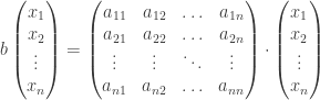
where $a_{ij} \in A$ . Write M for the RHS matrix; denoting $I$ for the $n\times n$ identity matrix, we get $(b\cdot I - M)\cdot \mathbf x = 0$ where $\mathbf x$ is the column vector $(x_1, \ldots, x_n)^t$ . Note that this relation holds in the ring C.

Now for every square matrix M with entries in any ring C, we can define its adjugate matrix N, which is a matrix of the same size with entries in C such that $MN = NM = \det(M)I$ . All entries of N can be obtained by polynomials in the entries of M with integer coefficients so this holds in any ring.

Applying this to our matrix $b\cdot I - M$ , we obtain $\det(b\cdot I - M)I\cdot \mathbf x = 0$ . In particular $0 = \det(b\cdot I - M)x_1 = \det(b\cdot I - M)$ . Expanding this determinant gives us a monic polynomial relation in b with coefficients in A. ♦

Easy Exercise

Prove that if $A\subseteq B \subseteq C$ are ring extensions such that B is finite over A, C is finite over B, then C is finite over A.

blue-lin

Consequences

The above gives us:

Proposition 1.

If $b_1, b_2 \in B$ are integral over A, so are $b_1 + b_2, b_1 b_2$ .

Proof

Consider the extensions

$A \subseteq A[b_1] \subseteq A[b_1, b_2].$

Since $b_2$ is integral over A, it is also integral over $A[b_1]$ , so both extensions are finite by the main proposition. Thus by the above exercise $A[b_1, b_2]$ is also a finite extension of A.

Since $b_1 + b_2, b_1 b_2 \in A[b_1, b_2]$ , by the main proposition they are integral over A. ♦

Example

We see that $\sqrt 2 + \sqrt[3] 3$ and $\sqrt 2 + \sqrt[3] 3 + \sqrt[5] 5$ are integral over $\mathbb Z$ since each summand is clearly integral over $\mathbb Z$ .

Definition.

By proposition 1, the set of $b\in B$ integral over A forms a ring extension of A contained in B. We call this the integral closure of A in B and denote it by $\mathrm{int. cl.}_A B$ .

We say B is integral over A if $\mathrm{int. cl.}_A B = B$ .

We say A is integrally closed in B if $\mathrm{int. cl.}_A B = A$ .

Next, we see that integrality is transitive.

Proposition 2.

Let $A\subseteq B\subseteq C$ be ring extensions, where $A\subseteq B$ is integral.

If $c\in C$ is integral over B, then it is integral over A.

Hence if C is integral over B and B is integral over A, then C is integral over A.

Proof

Since c is integral over B there are $b_0, b_1, \ldots, b_{n-1} \in B$ such that

$c^n + b_{n-1} c^{n-1} + \ldots + b_1 c + b_0 = 0.$

By the main proposition, we have a sequence of ring extensions, each finite over the previous.

$A \subseteq A[b_0] \subseteq A[b_0, b_1] \subseteq \ldots \subseteq A[b_0, \ldots, b_{n-1}] \subseteq A[b_0, \ldots, b_{n-1}, c]$

so $A[b_0, \ldots, b_{n-1}, c]$ is finite over A; again by the main proposition, c is integral over A. ♦

warning Recall that for a field extension $k\subseteq K$ , a finite extension is algebraic but the converse may not be true; heuristically, this is because we can attach infinitely many algebraic elements to k. This inspires the following.

Proposition 3.

If B is an A-algebra of finite type, and B is integral over A, then B is finite over A.

Proof

Write $B = A[b_0, \ldots, b_{n-1}]$ . In the extensions $A \subseteq A[b_0] \subseteq \ldots \subseteq A[b_0, \ldots, b_{n-1}] = B$ , each ring is finite over the previous. Hence B is finite over A. ♦

blue-lin

Normal Domains

In this section, for an integral domain A, $K := \mathrm{Frac} A$ denotes its field of fractions.

Definition.

We say A is a normal domain if it is integrally closed in K.

The normalization of A is the integral closure of A in K.

Exercise A

Prove that the normalization of A is a normal domain.

Note

In some books, A is called an integrally closed domain, but we consider it potentially confusing here. On the other hand, the term normal is used excessively in mathematics. However, in the context of commutative algebra this should not cause any confusion.

Example

Let $A = \mathbb Z[2i] = \{a + 2b\cdot i : a, b\in \mathbb Z\}$ where $i = \sqrt{-1}$ . Then $K = \mathbb Q[i]$ . Now A is not a normal domain because $i \in K$ is integral over A but does not lie in A.

One reason for defining normal domains lies in the following.

Proposition 4.

Let $A\subseteq B$ be integral domains, where $A$ is normal. For an integral $b\in B$ , consider it as an element of $\mathrm{Frac} B$ and take its minimal polynomial

$q(X) = X^n + c_{n-1} X^{n-1} + \ldots + c_0 \in K[X]$ .

Then $q(X) \in A[X]$ .

Proof

Find a monic polynomial $p(X) \in A[X]$ such that $p(b) = 0$ . Note that $q(X)$ divides $p(X)$ in $K[X]$ . Now pick a field extension $L\supseteq \mathrm{Frac} B$ in which $q(X)$ factors as a product of linear factors

$q(X) = (X - \alpha_1) \ldots (X - \alpha_n), \ \alpha_i \in L$ .

Since $p(\alpha_i) = 0$ each $\alpha_i$ is integral over A. Thus the coefficients of $q(X)$ are integral over A, being elementary symmetric polynomials in the $\alpha_i$ . Hence the coefficients of $q(X)$ lie in $\mathrm{int. cl.}_A K = A$ . ♦

However, to use the above result, we need a criterion for normal domains.

Proposition 5.

A UFD is a normal domain.

Proof

Let A be a UFD and suppose $\frac a b \in K$ is integral over A where a and b have no common prime factor. Pick $a_0, \ldots, a_{n-1} \in A$ such that

$(\frac a b)^n + a_{n-1} (\frac a b)^{n-1} + \ldots + a_0 = 0\implies a^n + a_{n-1}(a^{n-1}b) + \ldots + a_0(b^n) = 0.$

Then $b|a^n$ . Since a and b have no common prime factor, b is a unit so $\frac a b \in A$ . ♦

Examples

1. Let $b = \frac 1 {\sqrt 2} \in \mathbb C$ , which has minimal polynomial $X^2 - \frac 1 2$ over $\mathbb Q$ . Since $\mathbb Z$ is a UFD, it is a normal domain. Thus b is not integral over $\mathbb Z$ which solves our problem at the beginning of the article.

2. Let $A = \mathbb Z[2i]$ and $\alpha = \sqrt i$ . The minimal polynomial of $\alpha$ over $\mathrm{Frac} A$ is $X^2 - i = 0$ , which does not lie in $A[X]$ . On the other hand $\alpha$ is integral over A because $\alpha^4 + 1 = 0$ . This happens because A is not a normal domain.

Exercise B

1. Decide if each of the following is a normal domain. Find its normalization.

$\begin{aligned}\mathbb Z[X], \quad \mathbb Z[\sqrt 2],\quad, \mathbb Z[\sqrt 5], \quad \mathbb C[X, Y, Z],\quad \mathbb C[X, Y]/(Y^2 - X^3 + X),\\ \mathbb C[X, Y, Z]/(Y^2 - X^3 + X),\quad \mathbb C[X, Y]/(Y^2 - X^3),\quad \mathbb C[X, Y, Z]/(X^2 + Y^2 + Z^2).\end{aligned}$

[ Hint: conjecture and prove a result about $A[X]/(X^2 - f)$ , where $f\in A$ and A is a UFD in which 2 is invertible. ]

2. Consider $A\subset B$ where $A = \mathbb Z[2i][X]$ and $B = \mathbb Z[2i][X, Y]/(3Y^2 - 2X^3 - 1)$ . Is this an integral extension?

3. Let $f\in \mathbb Z[X, Y]$ . Prove that there is a $g \in \mathbb Z[X, Y] - \{0\}$ such that $fg \in \mathbb Z[X^{123}, Y^{789}]$ .

blue-lin

Posted in Advanced Algebra | Tagged field of fractions, finite extensions, integral closure, integral extensions, normal domains, rings, UFDs | 4 Comments

Commutative Algebra 38

Posted on April 26, 2020 by limsup

Artinian Rings

The main result we wish to prove is the following.

Theorem.

A ring A is artinian if and only if it is noetherian and $\dim A = 0$ , where $\dim$ denotes the Krull dimension.

Note

Recall that $\dim A = 0$ means all prime ideals of A are maximal.

Since the proof is long we will break it up into steps.

blue-lin

Artinian ⟹ Dim = 0

Step 1: An artinian integral domain A is a field.

Let $x \in A - \{0\}$ . From the sequence $(x) \supseteq (x^2) \supseteq (x^3) \supseteq \ldots$ we have $(x^n) = (x^{n+1})$ for some n > 0. Thus $x^n = x^{n+1}y$ for some $y\in A$ . Since A is a domain and $x\ne 0$ we have $xy = 1$ so x is a unit.

Step 2: An artinian ring A has finitely many maximal ideals.

Let $\Sigma$ be the collection of ideals of A of the form $\mathfrak m_1 \cap \ldots \cap \mathfrak m_k$ where $\mathfrak m_i \subset A$ are maximal ideals. Since A is artinian $\Sigma$ has a minimal element $\mathfrak a = \mathfrak m_1 \cap \ldots \cap \mathfrak m_k$ . By minimality for any maximal ideal $\mathfrak m$ we have $\mathfrak a \cap \mathfrak m = \mathfrak a$ and so $\mathfrak a \subseteq \mathfrak m$ . We claim that $\mathfrak m = \mathfrak m_i$ for some $1\le i \le k$ which would complete our claim.

Since $\mathfrak m$ and $\mathfrak m_i$ are all maximal it suffices to show $\mathfrak m \supseteq \mathfrak m_i$ for some i. Indeed if not we can pick $x_i \in \mathfrak m_i - \mathfrak m$ for $i=1,\ldots, k$ . Then

$x_1 \ldots x_k \in \mathfrak m_1 \ldots \mathfrak m_k \subseteq \mathfrak m_1 \cap \ldots \cap \mathfrak m_k = \mathfrak a \subseteq \mathfrak m$

a contradiction.

Step 3: An artinian ring A has finitely many prime ideals, all maximal.

For any prime ideal $\mathfrak p \subset A$ , $A/\mathfrak p$ is an artinian integral domain, hence a field by step 1. Thus $\mathfrak p$ is maximal so all prime ideals of A are maximal. By step 2, there are only finitely many of them.

Thus, we have shown that an artinian ring has Krull dimension 0. Since the connected components of Spec A are all singleton sets, we have proven:

Intermediate Result.

An artinian ring A is a finite product $A_1 \times \ldots \times A_k$ , where each $A_i$ is a local artinian ring with a unique prime ideal.

Our next target is noetherianness.

blue-lin

Artinian ⟹ Noetherian

By the intermediate result, we may assume A is a local artinian ring, with a unique prime ideal $\mathfrak p$ which is the nilradical of A. [ Recall (proposition 5 here) that in any ring, the nilradical is the intersection of all its prime ideals. ]

Step 4: $\mathfrak p$ is nilpotent.

We claim $\mathfrak p^N = 0$ for some N > 0. Note that this is not a trivial result: since $\mathfrak p$ is the nilradical, for each $x \in\mathfrak p$ we can find N such that $x^N = 0$ but we have to find an N which works for all x.

For that take $\mathfrak p \supseteq \mathfrak p^2 \supseteq \ldots$ . Since A is artinian $\mathfrak p^N = \mathfrak p^{N+1} = \ldots$ for some N>0. Write $\mathfrak a$ for this ideal so $\mathfrak a = \mathfrak a^2 = \ldots$ . It remains to show $\mathfrak a = 0$ .

If not, among all ideals $\mathfrak b$ such that $\mathfrak {ab} \ne 0$ , pick a minimal $\mathfrak b$ . Pick any $x\in \mathfrak b$ such that $x\mathfrak a \ne 0$ . Since $(x)\mathfrak a \ne 0$ minimality of $\mathfrak b$ forces $\mathfrak b = (x)$ . Also

$(x\mathfrak a)\mathfrak a = x\mathfrak a^2 = x\mathfrak a \ne 0 \implies x\mathfrak a = \mathfrak b = (x)$

by minimality of $\mathfrak b$ again. Thus $x = xy$ for some $y\in \mathfrak a$ . Since y is nilpotent we have $y^N = 0$ for some N; hence $x=0$ , a contradiction.

Step 5: An artinian ring A is noetherian.

Continuing step 4, we now have

$0 = \mathfrak p^N \subseteq \mathfrak p^{N-1} \subseteq \ldots \subseteq \mathfrak p \subseteq A.$

Each $\mathfrak p^i/\mathfrak p^{i+1}$ is an artinian A-module. Furthermore $\mathfrak p^i / \mathfrak p^{i+1}$ is a vector space over $A/\mathfrak p$ ; by exercise B.2 here this is artinian and hence finite-dimensional. Thus $\mathfrak p^i / \mathfrak p^{i+1}$ is a noetherian module over $A/\mathfrak p$ and hence over A (again by exercise B.2 here). This shows that A is noetherian.

blue-lin

Noetherian + Dim 0 ⟹ Artinian

Step 6: A noetherian ring A of Krull dimension 0 is artinian.

Since the connected components of Spec A are all singleton sets, A is a direct product of noetherian rings $A_1, \ldots, A_k$ , where each $A_i$ has a unique prime ideal. It suffices to prove each $A_i$ is artinian so we assume A is noetherian and has a unique prime ideal $\mathfrak p$ .

Since A is noetherian, $\mathfrak p$ has a finite generating set $x_1, \ldots, x_n$ . There is an M > 0 such that $x_i^M = 0$ for each i. It follows that $\mathfrak p^{nM} = 0$ . [ Indeed this ideal is generated by all $t = \prod x_i^{m_i}$ over all $m_1 + \ldots + m_n = nM$ , $m_i \ge 0$ . Since $m_i \ge M$ for some i, we have $t=0$ . ]

Let N = nM so that $\mathfrak p^N = 0$ . As above, form the sequence

$0 = \mathfrak p^N \subseteq \mathfrak p^{N-1} \subseteq \ldots \subseteq \mathfrak p \subseteq A.$

Each $\mathfrak p^i/\mathfrak p^{i+1}$ is now a noetherian vector space over $A/\mathfrak p$ so it is finite-dimensional. Thus it is also artinian over $A/\mathfrak p$ and hence over A. This shows that A is artinian. ♦

This completes our proof. Together with the previous article, we have:

Corollary 1.

Every artinian ring has a composition series and thus a well-defined length and set of composition factors.

warning Although all artinian rings are noetherian, there are artinian modules which are not noetherian, as we saw in the previous article.

Optional Note

For non-commutative rings, it is also true that a (left) artinian ring is (left) noetherian, but its proof is much more involved.

blue-lin

Special Case

Now suppose A is a reduced artinian ring. We factor

$A = A_1 \times \ldots \times A_k$

as above, where each $A_i$ is an artinian ring with a unique prime ideal $\mathfrak p_i$ . Since each $A_i$ is also reduced, its nilradical $\mathfrak p_i$ is zero so $A_i$ is a field. Hence we have shown:

Corollary 2.

The ring A is reduced and artinian if and only if it is isomorphic to a finite product of fields.

We also have the following special case.

Corollary 3.

Let A be an algebra over a field k such that $\dim_k A < \infty$ as a vector space. Then A is noetherian, $\dim A = 0$ and

$A = A_1 \times \ldots \times A_m$

where each $A_i$ has a unique prime ideal $\mathfrak p_i$ . Furthermore,

$m \le \dim_k A$ is the number of prime ideals of A;

if A is reduced then each $A_i$ is a finite field extension of k;

if A is reduced and k is algebraically closed, then each $A_i \cong k$ so $m = \dim_k A$ .

Note that in the context of algebraic geometry, if $A = k[V]$ for an affine k-scheme V (k algebraically closed), then each $A_i$ corresponds to a point $P\in V$ .

blue-lin

Posted in Advanced Algebra | Tagged artinian, krull dimension, nilradical, noetherian | Leave a comment

Minkowski Theory: Introduction

Picard Group of Number Rings

Geometric Example: Elliptic Curve Group

Properties of Dedekind Domains

Constructing Dedekind Domains

Valuation

Valuation in Geometry

Composition Series

Invertibility is Local

Dedekind Domains

Discrete Valuation Rings

Conditions for DVR

Fractional Ideals

Invertible Fractional Ideals

Picard Group

Localization

Catenary Rings

Clarifications

1. On Catenary Rings

2. Maximal Prime Chains in Catenary Rings

3. Catenary Rings Which Are Integral Domains

4. Dimension of Noetherian Rings

More Consequences of NNT

Height of an Ideal

Noether Normalization Theorem

Proof of Nullstellensatz

Consequences of NNT

Basic Definitions

Swapping Lemma

Transcendence Degree is Well-Defined

Transitivity

More on Integrality

Spectra of Integral Extensions

Consequences

Going Up Theorem

Integrality

Consequences

Normal Domains

Artinian Rings

Artinian ⟹ Dim = 0

Artinian ⟹ Noetherian

Noetherian + Dim 0 ⟹ Artinian

Special Case

Recent Posts

Archives

Categories

Meta

Pages