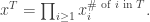
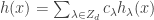
For now, we will switch gears and study the combinatorics of the matrices  and
and  where
where  run over all partitions of d>0. Eventually, we will show that there is a matrix K such that:

where J is the permutation matrix swapping  and its transpose. To achieve that, we will need to digress a little.

Young Tableaux
Let be any partition; we will use a Young diagram for comprising of boxes. A filling of is obtained by writing a positive integer in each box. The filling is called a semistandard Young tableau (SSYT) if the rows are weakly increasing and columns are strictly increasing. Finally, it is called a standard Young tableau (SYT) if the entries are a permutation of 1 to 
If  the following are examples:

is called the shape of a filling, while the tuple  where
where  is the number of occurrences of k, is called the type of the filling. Thus, the above 3 fillings all have shape (4, 3, 1); their types are (1, 3, 2, 1, 1), (2,2,2,0,1,1) and (1,1,1,1,1,1,1,1) respectively.
We will now describe an important operation to create new SSYTs.
Row Insertions
Given an SSYT P and positive integer k, we write  for the filling which has
  added to it in the following manner.
- First we add k to the first row. If k ≥ the rightmost entry, we add another square to the tableau and write k in it; this ends the process.
- Otherwise, starting from the rightmost entry and proceeding leftwards, we find the first square whose contents we can replace with k, while ensuring that the row is weakly increasing. In other words, we find the leftmost element which is greater than k, then swaps with k. If that square had content j, we say that k bumps out j.
- Now we proceed to add j to the next row, via the above process.
- If we finish all rows with square i left over, we add a row with a single square and write i in it.
As the reader may suspect, is always an SSYT (to be proved later).
Example
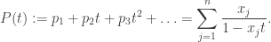
Suppose we have an SSYT with three rows: (1,1,2,4,5,6,6), (2,3,5,5,7) and (3,4,6); to add an element 3 to it, we proceed as follows, ending with a tableau with four rows. Thus, 3 bumps out 4 in the first row, which bumps out 5 in the second row, etc.

For convenience, we let  denote the set of squares whose contents were replaced (or added). Each square is denoted by
  , where i is the row number and j is the column number. In the above example, we obtain:
Basic Properties
Lemma 1. The replaced squares move to the left (weakly) as we proceed down the rows, i.e. if  , then
Proof
Suppose  ; consider the square directly below it. Either it is
  or it does not exist. In the latter case, we do not worry about
  In the former case, since
  is larger than the bumping number
  no square after
  can be bumped. ♦
Lemma 2. The resulting  is a semistandard Young tableau.
Proof
By construction, the rows of are weakly increasing so we need to show that its columns are strictly increasing. Suppose  bumps out
  ; since a number can only bump out something bigger, the number directly beneath
  (if it exists) is
What about the number above ? Suppose the bumped number in row  was
was  By lemma 1, we have
  . As was bumped out, the new entry at
  is
is  . Since
  , the new number at
  is also . ♦
Lemma 3. If  , then the replaced squares
  lie strictly to the left of
Proof
The proof is by induction on row. Say, on the first row,  bumps out
  in
in  , and bumps out in
  . Since
  and can only bump out something bigger, bumps out something strictly to the right of
  Since
Since  the induction may proceed onto the next row. ♦
Exercise
Prove that if  , then
  lie weakly to the right of
Lemma 4. Given an SSYT P and a corner box b (i.e. a box with no boxes to its right or below), there is a unique SSYT Q and positive integer k such that  and the additional box is on b.
Proof
Suppose the rightmost square of row r in P is . Remove it; since there are no boxes to its right or below, the subfilling from row r onwards is an SSYT. If we are on the top row, stop.
Otherwise, on the row above, find the rightmost square which is and replace it with  Note that such a square must exist since the square directly above is already
  Repeat until we reach the top row. ♦
Exercise
For each row in SSYT P below, remove the rightmost square and find the corresponding  such that

Exercise
Write a program in Python to perform row insertion and removal.


, where
for each


is called the shape of the tableau and its type is given by
where
is the number of times
appears.

is
. E.g. the above diagram gives

is symmetric.


with
, we have:
is left adjoint to multiplication by


are called the Littlewood-Richardson coefficients.

 is a graph which is directed, has no cycles, and there are only finitely many paths from a vertex to another. Given sets of n vertices:
 to
to  .
. of the graph has a weight
  which takes values in a fixed ring. Given a directed path
  from
from  to
to  let
let  be the product of the edges along the path
  for the sum of

 above, we compute the determinant of:
 where each
  for some permutation
  Furthermore we want the paths to be pairwise non-intersecting, i.e. no two paths contain a common vertex (not even at the endpoints). Now we can state the desired result.
 described above.
 ; each term is of the form:
 , the above term is a sum of terms of the form
 This is close to the desired result but here, the
  may intersect. Hence, we wish to show that the sum over all
  intersect, vanishes.
 be the collection of all such paths; for each
  we:
we: be the first vertex occurring as an intersection between
  ), after taking a total ordering for the set of vertices;
 );
); Now let
  be the same tuple of paths but with the tails of
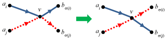
 , which is an involution since the corresponding triplet for
  is still
  and
and  have opposite signs. Denoting
  by
by  we have
  and so:

 be the transpose of

 is chosen to be
  and
and  in the respective cases.
 for all
  Observe that since
  , there is no harm increasing
  , so let us show the first. Before we begin, observe that the Schur polynomial can be written as:
 Indeed, this follows from the
  be large; we take the following graph.
 .
.
 are labelled
  for
for 
 , here is an example of paths connecting

 to
to  sums up to the complete symmetric polynomial
  . Thus the LHS is the desired determinant expression.
 to
to  . For a path to exist,
  must be the identity. Each collection of non-intersecting paths corresponds to a reverse SSYT of shape
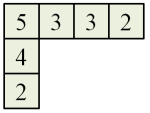
 of shape
  This is equal to the sum over all SSYT
  to be the minimum and maximum elements of the table respectively and replace each
  with
with  thus obtaining an SSYT). Thus the sum is
  ♦
♦
 of non-negative integers, define the following determinant, a polynomial in
  :
: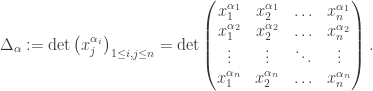
 , we also denote
  The following result is classical.
 Also, for any
  the polynomial
  is divisible by
 results in an exchange of two columns, which flips the sign of the determinant. Thus when
  ,
,  for all
  It remains to prove the first statement.
 and
and  are both homogeneous of degree
  so they are constant multiples of each other. Since the largest term (in lexicographical order) is
  on both sides, equality holds. ♦
 ; append zeros to it so that
  elements. Now define:
 is symmetric; note that it is homogeneous of degree
 . We have:
 is precisely the Schur polynomial
  ; this will be proven through the course of the article.
 and let
  ; we have:

 ; hence let us compare their coefficients of
  where
where  Since both sides are alternating polynomials, we may assume
  Now expand the LHS:
 , each term is of the form
  so the exponents of
  increases each exponent by at most 1. Thus to obtain
  ), then pick
  corresponds to a binary n-vector
  of weight r, such that
  is strictly decreasing. And the latter holds if and only if
  is a partition.
 we get:

 Successively applying Pieri’s formula gives:
 and the Young diagram for
  is obtained from
  boxes such that no two lie in the same row; the sum is over the set of all such
  Label the additional boxes in
  by
by  and take the transpose; we obtain an SSYT of shape
  and type
  ; here is one way we can successively add squares:

 in the above nested sum is
  This gives:
 , we get
  as desired. ♦
 :
:
 ) is taken over all partitions obtained by adding
  . Hence it holds in
  we get the second formula. ♦
 over all partitions
  if
if  ] We have an equality of formal power series:
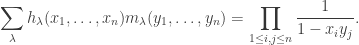
 and
and  to denote
  respectively. Also
  means
means 
 , there are only finitely many partitions of
  so we get a finite sum in
  . The eventual sum lies in
  , a formal power series in
 , we have
 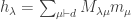 . Thus we need to show:
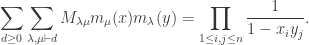

 in the expanded product. E.g. for
  and
and  , to obtain the term
  we can multiply:
 , and the coefficient of
  on the RHS is exactly
  This means RHS = LHS. ♦
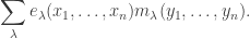

 Then the sets
 -bases of
 which takes
  for all
  Its kernel has a basis given by the monomial symmetric polynomials
  Now if
  and
and  we have
 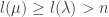 as well. Thus:
 is a basis of
  the set
  thus forms a basis of
  and the matrix
  is invertible, we see that
  also forms a basis of

 when we are confined to
 and
and  to be dual bases. As before, we have the following.
 is an orthonormal basis.
 However, the involution
  is no longer unitary. This can be checked for n=2, d=3. Here, we get
  and
and  A bit of computation then shows that
  which is not a unit vector. The reader should examine the proof to see why it does not carry over.
 indexed by
  and
and  If Cauchy’s identity holds for them:
 and
and  are dual bases with respect to the Hall inner product.
 and
and 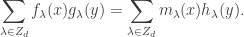
 is a basis of
  ; comparing dimensions, it suffices to show that the set spans this space.
 such that
  for all
 , where the
  is computed term-wise by taking
  as a power series in x with coefficients in
 ![\mathbb{Z}[\![ y ]\!]](https://s0.wp.com/latex.php?latex=%5Cmathbb%7BZ%7D%5B%5C%21%5B+y+%5D%5C%21%5D&bg=ffffff&fg=333333&s=0&c=20201002) ):
):
 as desired.
 , where the dual is taken over
  We have:
 with any
  In particular
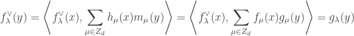
 of the formal ring. Recall that the sets
 .
.
 and
and  to be dual, i.e.
  where
where  is 1 if
  and 0 otherwise.
 for any

 , we have
 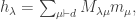 so
so  By definition
  for any partitions
  over all
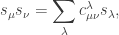
  We get:
 since the inner product is symmetric and
  By linearity,
 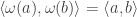 for any
  ♦
♦
 is the Kostka number, i.e. number of SSYT with shape
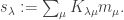
 and thus
  Note that
  where
where 

 , the Kronecker delta function (which takes 1 when
  and 0 otherwise).
 and
and  we have:

 as a matrix
  , we get
  ; since
  is invertible,
  so the
  form an orthonormal basis of
  Now apply the following.
 , i.e.
  If
If  is another orthonormal basis of
  then there is a permutation
  such that:
 for some
  We get:
 for some
  depending on
  for all
  The map
  gives a function
  Since the
  form a basis,
  for some permutation of
  We write this as
  where
where  has exactly one non-zero entry in each row and each column, and such an entry is
  Thus
Thus
 is upper-triangular with all 1’s on the main diagonal where
  is a permutation matrix swapping
  (so
(so  ). Hence:
 are non-negative, it follows that
  .
. for all


 and J is a permutation matrix, we have
  and
and 
 :
:
 and
and  :
:

 balls in it. Next, we number each ball as follows:
 ; label the balls 1, 2, … in order;
 for all
  and
and  ); let

 , look at all the balls in the current matrix containing k; this gives a diagonal zig-zag line, running from top-right to bottom-left. Between consecutive balls containing k, say at
  and
and  with
with 
 we place a ball at
  in the new matrix without any label. Working with our matrix of balls above, we obtain:
 be the matrix of non-negative integer entries such that
  is the number of balls in this new matrix. Now we label the balls in this new matrix as before, by starting from the top-left corner and proceeding left to right, top to bottom. In our working example, in the new matrix, we place 1 ball for k=3, 1 ball for k=4 and 2 balls for k=5. This gives the new matrix of balls:
 and
and  which is consistent with our RSK computation.
 the number of balls in the first matrix. Clearly there is nothing to show when
 ; let
; let  be the last element occurring in the two-row array
  corresponding to the matrix
  Consider the following.
 be the matrix equal to
 is the same as that of
  , but with one ball removed from
 obtained from its matrix balls is the same as that obtained by RSK.
 is obtained from matrix balls of
  then
then  and
and  is obtained from
  by attaching u to the corresponding extra square.
 and
and  and no other k occurs between rows
  or columns

 the k-th entry equals
  and the 1st to (k-1)-th entries are all
  On the other hand, the k-th entry of
  Also, note that the first row of
  Thus the first rows of P and Q are consistent with the RSK construction.
 , i.e. one at
  Note that
  and
and  is the transpose of
  All the remaining constructions are similarly transpose, with the rows and columns swapped.
 it suffices to prove invariance under
  This is via the Bender-Knuth involution.
 copies of
  copies of
  Now replace them by
  copies of
 is the number of SSYT of the shape
  if
if  .
. . Since
  , this is in fact an SYT and there are two possibilities.
 and
and  , no such tableau exists. Hence
 , then
  , i.e. for each
 .
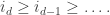
. must occur in the first
  is at least the number of these integers, i.e.
  This proves the inequality. If equality holds for all
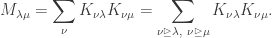

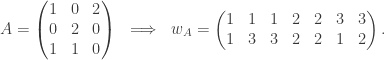
 of non-negative integers, with column sum
  and row sum
  We do not assume that
 ;
; , then
  (together with the first condition, this means the sequence of
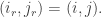
 .
. , let
, let  and
and  be the SSYT with the same shape as
  but with
  added to the extra box.
 ; the coloured cells on the left refer to the bumped cells, while those on the right are the additional cells attached to maintain the same shape.
 is an SSYT for each
 , then
  then
then  so by
so by  Since these include all occurrences of
  in
in  in the new cell for
  ♦
♦ , we have obtained (P, Q) of the same shape such that the type of P is
  gives a bijection:
 and perform reverse row-insertion from the corresponding square of P to obtain
  This gives us
  and a pair
 Now suppose
  along the way. The box removed for
  Hence in P, the bumped entries for
  are strictly to the right of
  (by
(by  ♦
♦


 be the number of SYT of shape
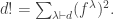
 , where
 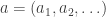 is a vector of non-negative integers such that only finitely many terms are non-zero. Thus
  and
and  are monomials but
  is not. Now for
  , consider the additive group
  of all sums
 ‘s may have infinitely many non-zero terms. E.g.
  is a perfectly valid element of
 such that
  for any permutation
  Note that each
 ; this gives us a homogeneous graded ring, called the formal ring of symmetric functions. E.g. in this ring, we have:
 taking
  gives a graded ring homomorphism
 be the map (graded ring homomorphism) taking
  Thus we get a sequence:
 one for each n.
 the maps
  are all isomorphisms; hence
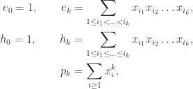
 etc, as before. Finally, the monomial symmetric polynomial
  over all
 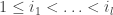 and
and  such that when sorted in decreasing order,
  becomes
  Note that
 , the above polynomials becomes their counterpart in
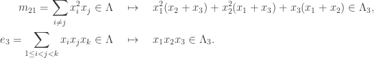

 shows that the same relations hold in
  for
for 

 for each n; this map does not commute with the projection
  For an easy example, say n=2, the map
  takes
takes  However, upon projecting to
  , the element
  while
while 
 Since
Since 
 to be that induced from
  for any
 since these hold in
 , although it seems natural to set
  As before, for a partition
 above since we have not defined
  For example if
 is
is  . Thus we have the following relation:
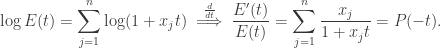
 we take the coefficient of
  on both sides and obtain Newton’s identities:
 for all k>n. With that, each
  can be written as a polynomial in
  with integer coefficients. E.g.
 as a polynomial in
  with rational coefficients. Thus we have:
![\displaystyle \Lambda_n \otimes_{\mathbb{Z}} \mathbb{Q} =\mathbb{Q}[p_1, p_2, \ldots, p_n],](https://s0.wp.com/latex.php?latex=%5Cdisplaystyle+%5CLambda_n+%5Cotimes_%7B%5Cmathbb%7BZ%7D%7D+%5Cmathbb%7BQ%7D+%3D%5Cmathbb%7BQ%7D%5Bp_1%2C+p_2%2C+%5Cldots%2C+p_n%5D%2C&bg=ffffff&fg=333333&s=0&c=20201002)
 -algebra in
  In particular,
  has basis given by
  for all
 Recall that the generating function for
  is
is  Hence:
 , taking the coefficient of
 with integer coefficients. E.g.
 as a polynomial in
  with rational coefficients.
 as a polynomial in:
 swaps
swaps  for
for  Looking at the expressions of
  in terms of
  the following is clear.
 , we have
 so this is clear. Suppose
  Apply
Apply  we have
  and so:
 for
for  so we get:
 as desired. ♦
 In the above diagram a → b means that b can be expressed as a polynomial in a with integer coefficients; the same holds for dotted arrows but now the polynomial may have rational coefficients.
 It turns out this has implications in the representation theory of the symmetric group
  We will (hopefully) get to talk about this beautiful result in a later article.