Polynomials and Representations XIII

Skew Diagrams

If we multiply two elementary symmetric polynomials $e_\lambda$ and $e_\mu$ , the result is just $e_\nu$ , where $\nu$ is the concatenation of $\lambda$ and $\mu$ sorted. Same holds for $h_\lambda h_\mu.$ However, we cannot express $s_\lambda s_\mu$ in terms of $s_\nu$ easily, which is unfortunate since the Schur functions are the “preferred” basis, being orthonormal. Hence, we define the following.

Definition. A skew Young diagram is a diagram of the form $\lambda/ \mu$ , where $\lambda$ and $\mu$ are partitions and $\lambda_i \ge \mu_i$ for each $i.$

E.g. if $\lambda = (7, 5, 3)$ and $\mu = (5, 2, 1),$ then

skew_young_diagram_example

Note that the same skew Young diagram can also be represented by $\lambda'/\mu'$ where $\lambda' = (8, 6, 4, 1)$ and $\mu' = (6, 3, 2, 1).$ These two Young diagrams are considered identical.

Definition. A skew semistandard Young tableau (skew SSYT) is a labelling of the skew Young diagram with positive integers such that each row is weakly increasing and each column in strictly increasing. Now $\lambda/\mu$ is called the shape of the tableau and its type is given by $\alpha$ where $\alpha_i$ is the number of times $i$ appears.

E.g. the following is a skew SSYT of the above shape. Its type is (4, 1, 1, 1).

skew_ssyt_example

blue-lin

Skew Schur Polynomials

Definition. The skew Schur polynomial corresponding to $\lambda/\mu$ is given by:

$\displaystyle s_{\lambda/\mu} := \sum_{\text{shape}(T) = \lambda/\mu} x^T$

where $x^T$ is $\prod_i x_i^{\text{\# of } i \text{ in } T}$ . E.g. the above diagram gives $x^T = x_1^4 x_2 x_3 x_4.$

The proof for the following is identical to the case of Schur polynomials.

Lemma. The skew Schur polynomial $s_{\lambda/\mu}$ is symmetric.

Indeed, one checks easily that the Knuth-Bendix involution works just as well for skew Young tableaux.

ssyt_bender-knuth_v2

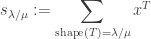
So the number of skew SSYT of shape $\lambda/\mu$ and type $\nu$ is unchanged when we swap $\nu_i$ and $\nu_{i+1}.$

Example

For $\lambda = (3, 2)$ and $\mu = (1)$ , we have:

skew_schur_polynomial_example

The following result explains our interest in studying skew Schur polynomials.

Lemma. The product of two skew Schur polynomials is a skew Schur polynoial.

For example, we have:

skew_schur_polynomial_product

It remains to express $s_{\lambda/\mu}$ as a linear combination of $s_\nu$ , where $|\nu| = |\lambda| - |\mu|.$

blue-lin

Littlewood-Richardson Coefficients

Recall that we have Pieri’s formula $h_r s_\lambda = \sum_\nu s_\nu$ , where $\nu$ is summed across all diagrams obtained by adding $r$ boxes to $\lambda,$ such that no two are on the same column. Repeatedly applying this gives us:

$\displaystyle h_\mu s_\lambda = \sum_{\nu_k} \sum_{\nu_{k-1}} \ldots \sum_{\nu_1} s_{\nu_k}$

where $\nu_0 := \lambda$ and $\nu_{i+1}$ is obtained from $\nu_i$ by adding $\mu_i$ boxes such that no two lie in the same column. Hence, the number of occurrences for a given skew Young diagram $\nu'$ is the number of skew SSYT’s with shape $\nu'$ and type $\mu.$

Example

If $\mu = (4, 2, 1)$ and $\lambda = (5, 4, 3)$ , here is one way of appending 4, 2, 1 boxes in succession:

skew_diagram_forming

which corresponds to the following skew SSYT:

skew_diagram_forming_2

This gives us the tool to prove the following.

Theorem. For any $f\in \Lambda^{(d)}$ with $d = |\lambda| - |\mu|$ , we have:

$\displaystyle \left< s_{\lambda/\mu}, f\right> = \left< s_\lambda, f s_\mu\right>$

so the linear map $s_\lambda \mapsto s_{\lambda/\mu}$ is left adjoint to multiplication by $s_\mu.$

Proof

It suffices to prove this for all $f = h_\nu$ where $\nu\vdash d.$ Since $\{h_\lambda\}$ is the basis dual to $\{m_\lambda\}$ , the LHS is the coefficient of $m_\nu$ in expressing $s_{\lambda/\mu}$ in terms of monomial symmetric polynomials. By definition of $s_{\lambda/\mu}$ , this is equal to the number of skew SSYTs with shape $\lambda/\mu$ and type $\nu$ ; we will denote this by $K_{\lambda/\mu, \nu},$ the skew Kostka coefficient.

By the reasoning above, when $h_\nu s_\mu$ is expressed as a linear combination of Schur functions, the coefficient of $s_\lambda$ is also $K_{\lambda/\mu, \nu}$ . Since the Schur functions are orthonormal, we are done. ♦

Note

The theorem is still true even when $\lambda_i \ge \mu_i$ does not all hold, if we take $s_{\lambda/\mu} = 0$ . Indeed, by reasoning with Pieri’s rule again, every Schur polynomial $s_\lambda$ occuring in $h_\nu s_\mu$ must have $\lambda_i\ge \mu_i$ for all $i.$

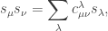
Definition. When we express:

$\displaystyle s_\mu s_\nu = \sum_{\lambda} c_{\mu\nu}^\lambda s_\lambda,$

the values $c_{\mu\nu}^\lambda = \left< s_\mu s_\nu, s_\lambda\right>$ are called the Littlewood-Richardson coefficients.

By the above theorem, this equals $\left< s_{\lambda/\mu}, s_\nu\right>.$ One can calculate this using the Littlewood-Richardson rule, which we will cover later.