Polynomials and Representations IX

Hall Inner Product

Let us resume our discussion of symmetric polynomials. First we define an inner product on d-th component $\Lambda^{(d)}$ of the formal ring. Recall that the sets

$\displaystyle \{h_\lambda : \lambda \vdash d\},\quad \{m_\lambda: \lambda \vdash d\}$

are both $\mathbb{Z}$ -bases of $\Lambda{(d)}$ .

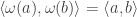
Definition. The Hall inner product

$\left<-, -\right> : \Lambda^{(d)} \times \Lambda^{(d)} \to \mathbb{Z},$

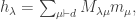
is defined by setting $\{h_\lambda\}_{\lambda \vdash d}$ and $\{m_\lambda\}_{\lambda\vdash d}$ to be dual, i.e. $\left< h_\lambda, m_\mu\right> := \delta_{\lambda\mu}$ where $\delta_{\lambda\mu}$ is 1 if $\lambda=\mu$ and 0 otherwise.

The introduction of the Hall inner product may seem random and uninspired, but it has implications in representation theory, which we will (hopefully) see much later. The following properties of the inner product are easy to prove.

Proposition.

The inner product is symmetric, i.e. $\left< a,b\right> = \left< b,a\right>$ for any $a,b\in \Lambda^{(d)}.$

The involution $\omega$ is unitary with respect to the inner product, i.e. $\left<\omega(a), \omega(b)\right> = \left<a, b\right>.$

Proof

For $\lambda\vdash d$ , we have $h_\lambda = \sum_{\mu\vdash d} M_{\lambda\mu} m_\mu,$ so $\displaystyle\left< h_\lambda, h_\mu\right> = M_{\mu\lambda}.$ By definition $M_{\mu\lambda} = M_{\lambda\mu}$ for any partitions $\lambda$ and $\mu$ . Thus the Hall inner product is symmetric.

Next, $\Lambda^{(d)}$ has bases given by $\{h_\lambda\}$ and $\{e_\lambda\}$ over all $\lambda \vdash d.$ We get:

$\displaystyle \left< \omega(h_\lambda), \omega(e_\mu)\right> = \left< e_\lambda, h_\mu\right> = N_{\lambda\mu}.$

which is equal to $\left< h_\lambda, e_\mu\right>$ since the inner product is symmetric and $N_{\lambda\mu} = N_{\mu\lambda}.$ By linearity, $\left<\omega(a), \omega(b)\right> = \left<a, b\right>$ for any $a,b \in \Lambda^{(d)}.$ ♦

In the next section, we will see that the inner product is positive-definite. Even better, we will explicitly describe an orthonormal basis which lies in $\Lambda.$

blue-lin

Schur Polynomials – An Orthonormal Basis

Recall that we have, in $\Lambda$ ,

$\mathbf h = \mathbf M \mathbf m, \qquad \mathbf M = \mathbf K^t \mathbf K,$

where $\mathbf K = (K_{\lambda\mu})$ is the Kostka number, i.e. number of SSYT with shape $\lambda$ and type $\mu.$

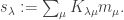
Definition. For each partition $\lambda$ , the Schur polynomial is defined as:

$s_\lambda := \sum_{\mu} K_{\lambda\mu} m_\mu.$

Written vectorially, this gives $\mathbf s = \mathbf K\mathbf m$ and thus $\mathbf h = \mathbf K^t \mathbf s.$ Note that $s_\lambda \in \Lambda^{(d)}$ where $d:=|\lambda|.$

For each n>0, the image of $s_\lambda$ in $\Lambda_n^{(d)}$ is also called the Schur polynomial; we will take care to avoid any confusion.

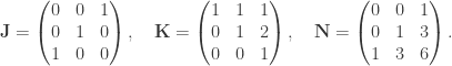
Example.

Consider the case of d=3. We have:

$\mathbf K = \begin{pmatrix} 1 & 1 & 1 \\ 0 & 1 & 2 \\ 0 & 0 & 1\end{pmatrix}\implies \begin{aligned} s_3 &= m_3 + m_{21} + m_{111},\\ s_{21} &= m_{21} + 2m_{111},\\ s_{111} &= m_{111}.\end{aligned}$

We then have:

Proposition. The polynomials $\{s_\lambda : \lambda \vdash d\}$ form an orthonormal basis of $\Lambda^{(d)},$ i.e. $\left<s_\lambda, s_\mu\right> = \delta_{\lambda\mu}$ , the Kronecker delta function (which takes 1 when $\lambda = \mu$ and 0 otherwise).

Proof

From $\mathbf s =\mathbf K\mathbf m$ and $\mathbf h = \mathbf K^t \mathbf s$ we have:

$\left< s_\lambda, h_\mu\right> = \left< \sum_\nu K_{\lambda\nu} m_\nu, h_\mu\right> = \sum_\nu K_{\lambda\nu}\delta_{\nu\mu} = K_{\lambda\mu},$

$\left< s_\lambda, h_\mu\right> = \left< s_\lambda, \sum_\nu K_{\nu\mu} s_\nu \right> = \sum_\nu K_{\nu\mu}\left< s_\lambda, s_\nu\right>.$

Treating $\left< s_\lambda, s_\nu\right>$ as a matrix $\mathbf A$ , we get $\mathbf A \mathbf K= \mathbf K$ ; since $\mathbf K$ is invertible, $\mathbf A = \mathbf I$ so the $s_\lambda$ are orthonormal. ♦

Corollary. The Hall inner product on $\Lambda^{(d)}$ is positive-definite.

blue-lin

Further Results on Schur Polynomials

Since $\{s_\lambda\}_{\lambda \vdash d}$ form an orthonormal basis of $\Lambda^{(d)},$ so do $\{\omega(s_\lambda)\}_{\lambda \vdash d}.$ Now apply the following.

Lemma. Suppose $A$ is a finite free abelian group with orthonormal basis $(v_i)_{i=1}^n$ , i.e. $\left< v_i, v_j\right> = \delta_{ij}.$ If $(w_i)_{i=1}^n$ is another orthonormal basis of $A,$ then there is a permutation $\sigma$ of $\{1,\ldots, n\}$ such that:

$w_i = \pm v_{\sigma(i)}, \quad \text{ for } i=1,\ldots, n.$

Thus, unlike vector spaces over a field, an orthonormal basis of a finite free abelian group is uniquely defined up to permutation and sign.

Proof

Fix $i$ and we have $w_i = \sum_{j=1}^n c_{ij} v_j$ for some $c_{ij} \in \mathbb{Z}.$ We get:

$1 = \left< w_i, w_i\right> = \sum_{j=1}^n c_{ij}^2.$

Thus $c_{ij_0} = \pm 1$ for some $j_0$ depending on $i$ , and $c_{ij} = 0$ for all $j \ne j_0.$ The map $i\mapsto j_0$ gives a function $\sigma : \{1,\ldots,n\} \to \{1, \ldots, n\}.$ Since the $\{w_i\}$ form a basis, $\sigma$ is a bijection. ♦

Thus $\omega(s_\lambda) = \pm s_{\sigma(\lambda)}$ for some permutation of $\{\lambda : \lambda \vdash d\}.$ We write this as $\omega(\mathbf s) = \mathbf W \cdot \mathbf s$ where $\mathbf W$ has exactly one non-zero entry in each row and each column, and such an entry is $\pm 1.$ Thus

$\begin{aligned}\mathbf h = \mathbf K^t \mathbf s &\overset {\omega} \implies \mathbf e = \mathbf K^t \omega(\mathbf s)= \mathbf K^t \mathbf W\mathbf s = \mathbf K^t \mathbf W \mathbf K \mathbf m\\ &\implies \mathbf N = \mathbf K^t \mathbf W\mathbf K.\end{aligned}$

Now we saw earlier that $\mathbf J\mathbf N$ is upper-triangular with all 1’s on the main diagonal where $\mathbf J$ is a permutation matrix swapping $\lambda$ with $\overline\lambda$ (so $\mathbf J^2 = \mathbf I$ ). Hence:

$\mathbf J \mathbf K^t \mathbf W \mathbf K = \begin{pmatrix}1 & \ldots & {\small \ge 0} \\0 & \ddots & \vdots \\0 & 0 & 1 \end{pmatrix} \implies \mathbf J \mathbf K^t =\begin{pmatrix}1 & \ldots & {\small \in \mathbb{Z}} \\0 & \ddots & \vdots \\0 & 0 & 1 \end{pmatrix} \mathbf W^{-1}.$

Since all entries of $\mathbf J \mathbf K^t$ are non-negative, it follows that $\mathbf W$ is a permutation matrix. And since $\mathbf K$ is also upper-triangular with 1’s on the main diagonal, we have $\mathbf W = \mathbf J$ .

blue-lin

Summary

Thus we have shown:

$\omega(s_\lambda) = s_{\overline\lambda}$ for all $\lambda \vdash d.$

$\mathbf M = \mathbf K^t \mathbf K \implies \mathbf h = \mathbf K^t \mathbf K \mathbf m.$

$\mathbf N = \mathbf K^t \mathbf J \mathbf K \implies \mathbf e = \mathbf K^t \mathbf J \mathbf K \mathbf m.$

The second and third relations can also be written as:

$\displaystyle M_{\lambda\mu} = \sum_{\nu \trianglerighteq \lambda,\, \nu\trianglerighteq \mu } K_{\nu\lambda} K_{\nu\mu},\qquad N_{\lambda\mu} = \sum_{\lambda\trianglelefteq \nu\trianglelefteq \overline\mu} K_{\nu\lambda} K_{\overline\nu \mu}.$

Also since $\det\mathbf K = 1$ and J is a permutation matrix, we have $\det \mathbf M = 1$ and $\det \mathbf N = \pm 1.$

Example

Consider the case d=3. Check that $\mathbf N = \mathbf K^t \mathbf J \mathbf K$ :

$\mathbf J = \begin{pmatrix} 0 & 0 & 1 \\ 0 & 1 & 0\\ 1 & 0 & 0\end{pmatrix}, \quad \mathbf K = \begin{pmatrix} 1 & 1 & 1 \\ 0 & 1 & 2 \\ 0 & 0 & 1\end{pmatrix}, \quad \mathbf N = \begin{pmatrix} 0 & 0 & 1 \\ 0 & 1 & 3 \\ 1 & 3 & 6\end{pmatrix}.$