Polynomials and Representations V

It was clear from the earlier articles that n (number of variables $x_1, \ldots, x_n$ ) plays a minimal role in the combinatorics of the symmetric polynomials. Hence, removing the parameter n turns out to be quite convenient; the process gives us the formal ring of symmetric functions.

Concrete Definition of Ring Λ

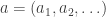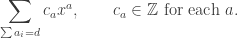
Consider the set of all monomials $x^a := x_1^{a_1} \ldots x_m^{a_m}$ , where $a = (a_1, a_2, \ldots)$ is a vector of non-negative integers such that only finitely many terms are non-zero. Thus $x_1 x_2$ and $x_1 x_2^2 x_3^3$ are monomials but $x_1 x_2 x_3 \ldots$ is not. Now for $d = 0,1,2,\ldots$ , consider the additive group $C_d$ of all sums

$\displaystyle\sum_{\sum a_i = d} c_a x^a, \qquad c_a \in \mathbb{Z} \text{ for each } a.$

Though each $a$ has only finitely many non-zero terms, the collection of all $c_a$ ‘s may have infinitely many non-zero terms. E.g. $x_1 + 2x_3 + 3x_5 + 4x_7 + \ldots$ is a perfectly valid element of $C_1.$

Now let $\Lambda^{(d)}$ be the subgroup of all $\sum_a c_a x^a \in C_d$ such that $c_a = c_{\sigma(a)}$ for any permutation $\sigma$ of $\{1,2,\ldots\}.$ Note that each $\Lambda^{(d)}$ is a finite free abelian group with basis elements given by:

$\begin{aligned} \Lambda^{(0)} &\longrightarrow \left\{1\right\},\\ \Lambda^{(1)} &\longrightarrow \left\{\sum_{i\ge 1} x_i\right\}, \\ \Lambda^{(2)} &\longrightarrow \left\{\sum_{i\ge 1} x_i^2, \sum_{1\le i<j} x_i x_j\right\},\\ \Lambda^{(3)} &\longrightarrow \left\{\sum_{i\ge 1} x_i^3, \sum_{\substack{i,j\ge 1 \\i\ne j}} x_i^2 x_j, \sum_{1\le i< j< k} x_i x_j x_k\right\}. \end{aligned}$

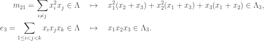
Let: $\Lambda := \oplus_{d=0}^\infty \Lambda^{(d)}$ ; this gives us a homogeneous graded ring, called the formal ring of symmetric functions. E.g. in this ring, we have:

$\left(\sum_{i=1}^\infty x_i\right)^2 = \left(\sum_{i=1}^\infty x_i^2\right) + 2\left( \sum_{1\le i < j} x_i x_j\right).$

For each n, the map $\Lambda^{(d)} \to \Lambda_n^{(d)}$ taking $x_{n+1}, x_{n+2}, \ldots \mapsto 0$ gives a graded ring homomorphism $\Lambda \to \Lambda_n.$

Abstract Definition of Λ

Here is an alternate definition: let $\Lambda_n \to \Lambda_{n-1}$ be the map (graded ring homomorphism) taking $x_n \mapsto 0.$ Thus we get a sequence:

$\ldots \longrightarrow \Lambda_{n+1} \longrightarrow \Lambda_n \longrightarrow \ldots \longrightarrow \Lambda_1 \longrightarrow 0.$

Now $\Lambda$ is defined to be the inverse limit of this sequence, which gives us a graded ring and a set of graded maps $\Lambda \to \Lambda_n,$ one for each n.

Note that if $n\ge d,$ the maps $\ldots \to \Lambda_{n+1}^{(d)} \to \Lambda_{n}^{(d)}$ are all isomorphisms; hence $\Lambda^{(d)} \to \Lambda_n^{(d)}$ is also an isomorphism.

blue-lin

Symmetric Polynomials in Λ

We define the following in $\Lambda$ , also called the elementary symmetric polynomial, complete symmetric polynomial and the power sum symmetric polynomial.

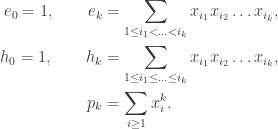
$\displaystyle\begin{aligned} e_0 = 1,\qquad e_k &= \sum_{1 \le i_1 < \ldots < i_k} x_{i_1} x_{i_2} \ldots x_{i_k},\\ h_0 = 1,\qquad h_k &= \sum_{1 \le i_1 \le \ldots \le i_k} x_{i_1} x_{i_2} \ldots x_{i_k},\\ \qquad p_k &= \sum_{i\ge 1} x_i^k.\end{aligned}$

For a partition $\lambda$ , we also define $e_\lambda := e_{\lambda_1} \ldots e_{\lambda_l}$ etc, as before. Finally, the monomial symmetric polynomial $m_\lambda$ is the sum of all $x_{i_1}^{a_1} x_{i_2}^{a_2} \ldots x_{i_l}^{a_l},$ over all 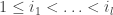$1 \le i_1 < \ldots < i_l$ and $(a_1, \ldots a_l)$ such that when sorted in decreasing order, $(a_i)$ becomes $(\lambda_i).$ Note that $\deg(m_\lambda) = |\lambda|.$

When projected via $\Lambda \to \Lambda_n$ , the above polynomials becomes their counterpart in $\Lambda_n.$ For example

$\displaystyle \begin{aligned} m_{21} = \sum_{i\ne j} x_i^2 x_j \in \Lambda \quad &\mapsto \quad x_1^2(x_2 + x_3) + x_2^2 ( x_1 + x_3)+ x_3(x_1 + x_2) \in \Lambda_3,\\ e_3 = \sum_{1\le i < j< k} x_i x_j x_k \in \Lambda \quad&\mapsto\quad x_1 x_2 x_3 \in \Lambda_3.\end{aligned}$

Rewriting Earlier Results

We thus have the following:

$\displaystyle \begin{aligned} e_\lambda &= \sum_{\mu \vdash d} N_{\lambda\mu} m_\mu,\\ h_\lambda &= \sum_{\mu\vdash d} M_{\lambda\mu} m_\mu, \end{aligned}$

where $d = |\lambda|.$ Indeed, the above relations hold in $\Lambda_n^{(d)}$ for any n and d; when $n\ge d,$ the isomorphism $\Lambda^{(d)} \cong \Lambda_n^{(d)}$ shows that the same relations hold in $\Lambda.$ Similarly, the identities from earlier can be copied over verbatim by projecting to $\Lambda_n^{(k)}$ for $n\ge k.$

$\displaystyle\begin{aligned} e_0 h_k - e_1 h_{k-1} + \ldots + (-1)^k e_k h_0 &=0,\\ e_{k-1}p_1 - e_{k-2}p_2 + \ldots + (-1)^{k-1}e_0 p_k &= ke_k, \\ h_{k-1}p_1 + h_{k-2}p_2 + \ldots + h_0 p_k &= kh_k.\end{aligned}.$

blue-lin

Duality in Λ

Recall that we have an involution $\omega:\Lambda_n \to \Lambda_n$ for each n; this map does not commute with the projection $\Lambda_{n+1} \to \Lambda_{n+1}.$ For an easy example, say n=2, the map $\omega : \Lambda_3 \to \Lambda_3$ takes $e_3 \mapsto h_3.$ However, upon projecting to $\Lambda_2$ , the element $e_3 \mapsto 0$ while $h_3 \mapsto \ne 0.$

This can be overcome by taking $n\ge d.$ Since $\omega$ is graded, we thus have the following:

commutative_diagram_formal_ring_d

The vertical lines are isomorphisms and the diagram commutes.

Definition. For each $d\ge 0$ , we define the involution $\omega : \Lambda^{(d)} \to \Lambda^{(d)}$ to be that induced from $\omega: \Lambda_n^{(d)}\to \Lambda_n^{(d)}$ for any $n\ge d.$

Note that in Λ, we have:

$\omega(e_k) = h_k, \quad\omega(h_k) = e_k, \quad\omega(p_k) = (-1)^{k-1}p_k$

for all $k\ge 1$ since these hold in $\Lambda_n^{(k)}$ for any $n\ge k.$

blue-lin