Mathematics and Such

Estimating Sums Via Integration

Posted on November 25, 2011 by limsup

Background required : calculus, specifically integration

By representing a sum $\sum_{i=1}^n a_i$ as an area, it is often possible to estimate its size by approximating it with the area underneath a curve.

For example, suppose we wish to compute the sum $b_n = 1 + \frac 1 2 + \frac 1 3 + \dots + \frac 1 n$ . There’s no known closed formula for b_n but we can get a pretty good grasp of its size in terms of n. Consider the graph of y = 1/x:

(Diagram edited from a graph plotted by wolframalpha.)

In both instances, the sum 1 + 1/2 + … + 1/n represents the area of the red region. From the diagram, it’s clear that this sum is at most $1 + \int_1^n \frac 1 x dx = 1 + \log n$ and at least $\int_1^{n+1} \frac 1 x dx = \log(n+1)$ . Thus:

$\log(n+1) \le b_n = 1 + \frac 1 2 + \dots + \frac 1 n \le 1 + \log n.$

In particular $b_n - \log n \le 1$ and it represents the area of the “white space” from x=1 to x=n on the left graph above. Since $b_n - \log n$ is an increasing sequence which is bounded from above, it must converge to some value. This is known as Euler’s gamma constant and an entire book has been written on it.

Anyway, we now know the following.

The sequence 1 + 1/2 + 1/3 + … + 1/n diverges to infinity and 1 + 1/2 + 1/3 … + 1/n – log(n) converges to a real number < 1.

By the same token, if s > 1 is a real number, we have:

$\int_1^{n+1} x^{-s} dx \le 1 + \frac 1 {2^s} + \frac 1 {3^s} + \dots + \frac 1 {n^s} \le 1 + \int_1^n x^{-s} dx.$

The LHS is $(s-1)^{-1} (1 - (n+1)^{-s+1})$ and the RHS is $1 + (s-1)^{-1}(1 - n^{-s+1})$ . In particular, since the sum is bounded above by 1 + 1/(s-1) it must converge!

If s>1 is a real number, then $1 + 1/2^s + 1/3^s + \dots + 1/n^s$ converges as $n\to \infty$ .

Stirling’s Approximation

Using this technique, we can also approximate n!, or rather, log(n!) = log(1) + log(2) + … + log(n). We shall approximate this sum with the area under the curve y = log(x) from x=1 to x=n. Via integration by parts, we have:

$\int \log x \cdot dx = x(\log x - 1) + c.$

So the sum log(1) + … + log(n) is about n(log n – 1) and

$n! \approx e^{n(\log n -1)} = \left( \frac n e\right)^n.$

A more precise analysis would give us $n! \approx \sqrt{2\pi n} (\frac n e)^n$ , but we won’t go into that detail.

In summary, sums are generally much more difficult to compute than integrals (by that, we mean partial sums of the form $b_n = a_1 + a_2 + \dots + a_n$ ). For example, consider the infinite sum $1 + 1/2^k + 1/3^k + \dots$ where k>1 is a fixed integer. For even k, there is a nice closed form for it: specifically it is a rational multiple of $\pi^k$ . The details of that would be another story for another day. For now, it suffices to say that integrals are a useful means to approximate sums.

Posted in Notes | Tagged basic, calculus, integration, notes, sums | Leave a comment

Matrices and Linear Algebra

Posted on November 24, 2011 by limsup

Background recommended : coordinate geometry

Here I thought I’d give an outline of linear algebra and matrices starting from a more axiomatic viewpoint, instead of merely giving rules of computation – the way it’s usually taught in school. The materials here are not really Olympiad-type of mathematics, but if you’ve always wondered why matrix multiplication is defined the way it is, you’ll hopefully get it by the end of this post. Purpose of this post:

introduction to axiomatic reasoning for students (no background is required since everything is derived from definitions, but it helps to keep the geometric picture in mind);
explain the purpose behind matrix operations.

Note: please try to do all the exercises to get a feel of the axiomatic approach.

The Object

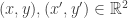
Our object of interest is $\mathbb R^2$ , which is the set of all pairs (x, y), where x, y are real. The pairs (x, y) and (x’, y’) are considered equal if and only if x=x’ and y=y’. E.g. (1, -1), (2.5, -1), (√2, 0), … are examples of (distinct) elements of $\mathbb R^2$ . Bear in mind that the underlying idea for (x, y) is a point on the plane with the corresponding coordinates.

Next, we shall define the following operations on $\mathbb R^2$ .

Addition : given $(x,y), (x',y') \in \mathbb R^2$ , the sum of these two pairs is defined to be $(x,y) + (x', y') = (x+x', y+y') \in \mathbb R^2$ . E.g. (-1, 3) + (5, 10.3) = (4, 13.3).
Multiplication by scalar : given any real number c and $(x,y) \in \mathbb R^2$ , the product between them is defined to be $c \times (x,y) = (cx, cy)$ . E.g. 1.5 × (-1, 2) = (-1.5, 3). Later, we will drop the × for brevity.
We will not define multiplication between elements of $\mathbb R^2$ .

All in all, totally intuitive concepts. If you draw the points on a plane, you’ll immediately see the geometric interpretation: if points A and B corresponds to (x, y) and (x’, y’) on the Cartesian plane, then the sum corresponds to a point C such that OACB is a parallelogram, where O = (0,0) is the origin.

Before I forget, for convenience, we will also define subtraction in terms of addition and multiplication: for any v, w in $\mathbb R^2$ , we define v – w = v + (-1)w. Note that each of the elements v, w is a pair of numbers. Clearly, the definition just means (x, y) – (x’, y’) = (x–x’, y–y’). You might wonder why I didn’t just say so; as a matter of fact, though it’s probably easier just to say (x, y) – (x’, y’) = (x–x’, y–y’), I was following the philosophy of having as few basic (atomic) definitions as possible.

The Functions

Next, we will describe what kind of functions $f:\mathbb R^2 \to \mathbb R^2$ are of interest to us. This will be a recurring theme throughout algebra and higher mathematics (and even object-oriented programming!) : you study the objects as well as the “nice” functions between them. Since we had defined a structure on $\mathbb R^2$ , clearly our f is expected to respect this structure.

A function $f:\mathbb R^2 \to \mathbb R^2$ is said to be linear if for any v and w in $\mathbb R^2$ and real number c, we have

$f(\mathbf{v} + \mathbf{w}) = f(\mathbf{v}) + f(\mathbf{w})$ ;

$f(c \times \mathbf{v}) = c\times f(\mathbf{v})$ .

Geometrically, if we have a line l on the plane $\mathbb R^2$ , then l gets mapped to f(l) which is also a line (can you prove it?). That’s the reason behind the name linear.

Basic Exercise : prove the following explicitly (with only the definitions/materials we’ve covered so far).

If f is linear then we must have f(0) = 0 (where 0 = (0,0)) as well as f(v–w) = f(v)-f(w).
f is injective if and only if we cannot a v, where v ≠ 0, such that f(v) = 0.
The function which takes all v in $\mathbf R^2$ to the zero element 0 is linear.
If f and g are linear functions $\mathbf R^2 \to \mathbf R^2$ , then the new function $h : \mathbb R^2 \to \mathbb R^2$ which is defined by h(v) := f(v) + g(v) is also linear.
Same as 4., but now replace h with the function h(v) = f(g(v)).
If f is linear and c is any real number, define a new function $h:\mathbb R^2 \to \mathbb R^2$ via h(v) = c × f(v). Prove that h is linear.

Properties 4-6 suggest that we can have operations among linear functions! In other words, we have functions which take in linear functions, and output another linear function. That’s not so weird if you think about it, since in algebra we can add and multiply polynomials (which are functions themselves).

Definition : Let $f, g : \mathbb R^2 \to \mathbb R^2$ be linear functions and c be a real number. Define the following:

f+g is the ‘h’ function defined in exercise 4 above.

f×g is the ‘h’ function defined in exercise 5.

c×f is the ‘h’ function defined in exercise 6.

In short, we can “add” or “multiply” two linear functions to give another. And we can multiply a linear function by a real number to obtain another linear function.

Matrices

Note that we’ve yet to see a single concrete example of a linear function. This is where matrices come in handy; we will also see that multiplication of two linear functions is non-commutative! In other words f×g and g×f are different in general.

The key property we will prove is this: fix the two elements $\mathbf{e}_1 = (1,0), \mathbf{e}_2 = (0,1) \in \mathbb R^2$ .

If $f, g : \mathbb R^2 \to \mathbb R^2$ are linear functions such that $f(\mathbf{e}_1) = g(\mathbf{e}_1)$ and $f(\mathbf{e}_2) = g(\mathbf{e}_2)$ , then f = g.
On the other hand, for any two elements $\mathbf{v}_1, \mathbf{v}_2 \in \mathbb R^2$ , there is a linear f such that $f(\mathbf{e}_1) = \mathbf{v}_1, f(\mathbf{e}_2) = \mathbf{v}_2$ .

[ In other words, the linear function f is uniquely determined by a pair of elements $\mathbf{v}_1, \mathbf{v}_2 \in \mathbb R^2$ . Note that since each of v₁ and v₂ is a pair of real numbers, we’re really looking at 4 real numbers here. ]

Proof. Suppose f, g satisfy $f(\mathbf{e}_1) = g(\mathbf{e}_1)$ and $f(\mathbf{e}_2) = g(\mathbf{e}_2)$ . Now any element of $\mathbb R^2$ is of the form v = (x, y) = x × e₁ + y × e₂ from which we get:

$f(\mathbf v) = f(x \mathbf e_1 + y \mathbf e_2) = x \times f(e_1) + y \times f(e_2) = x \times g(e_1) + y \times g(e_2) = g(x \mathbf e_1 + y \mathbf e_2) = g(\mathbf v).$

[ Make sure you understand each step thoroughly! ]

Thus f = g. For the second property, again we can write v = (x, y) and we simply define $f : \mathbb R^2 \to \mathbb R^2$ via

$f( (x,y) ) = x \times \mathbf v_1 + y\times \mathbf v_2.$

[ Test of concept: why are there double brackets around “x,y” ? ]

We need to show that this f is linear, e.g. to show f( (x,y) + (x’,y’) ) = f( (x,y) ) + f( (x’, y’) ) , we have:

By definition, RHS 1st term = x × v₁ + y × v₂ and RHS 2nd term = x’ × v₁ + y’ × v₂.
LHS = f( (x+x’, y+y’) ) = (x+x’) × v₁ + (y+y’) × v₂ = (x × v₁) + (x’ × v₁) + (y × v₂) + (y’ × v₂).

The remaining condition: f(c(x, y)) = c × f(x, y) is left as an exercise for the reader. ♦

Concrete Example. Suppose we pick elements v₁ = (2, 3) and v₂ = (-1, 4). The corresponding linear function f is given by:

f( (x, y) ) = x × (2,3) + y × (-1,4) = (2x–y, 3x+4y).

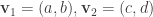Given a linear map $f : \mathbb R^2 \to \mathbb R^2$ , which corresponds to $\mathbf v_1$ and $\mathbf v_2$ , write $\mathbf v_1 = (a, b), \mathbf v_2 = (c, d)$ . The 2-by-2 matrix corresponding to f is then defined to be the 2-by-2 table of values:

$M = \begin{pmatrix} a & c \\ b & d \end{pmatrix}.$

Thus there is a one-one correspondence between linear maps and 2-by-2 matrices.

Now the following exercises will explain the definition for matrix multiplication.

Important exercises. Let f, g, h be any linear maps and M, N, P be the corresponding 2-by-2 matrices (respectively).

We have already seen that f+g is linear. Write the matrix corresponding to it by examining the images of e₁ = (1,0) and e₂ = (0,1).
Likewise do the same for the linear maps fg and c × f. Verify that the matrix corresponding to fg is precisely the matrix multiplication M × N.
Prove the following equality of linear maps, by examining the images of various $\mathbf v \in \mathbb R^2$ .

f(g + h) = fg + fh;
f(gh) = (fg)h.

Use exercise 3 to prove the following:

For any matrices A, B, C, we have A(B + C) = AB + AC.
For any matrices A, B, C, we have A(BC) = (AB)C.

Qualitatively, this also explains why multiplication of matrices don’t commute. This follows from the fact that matrix multiplication corresponds to function composition, and generally function compositions don’t commute (try putting on the shoes before putting on the socks).

Long but insightful exercise. Develop the whole theory in greater generality. Start with $\mathbb R^n$ for general positive integer n. Consider linear functions $f : \mathbb R^m \to \mathbb R^n$ for positive integers m and n. We can add and compose linear functions which are of “appropriate dimensions”. E.g. if $f : \mathbb R^m \to \mathbb R^n$ and $g : \mathbb R^n \to \mathbb R^k$ , then $gf : \mathbb R^m \to \mathbb R^k$ . Thus prove that matrix multiplication is, in general, associative, and distributive over addition.

Posted in Extra | Tagged axiomatic, basic, linear algebra, notes | Leave a comment

Sample Problem Solving + Homework Hints

Posted on November 21, 2011 by limsup

In this post, I’ll talk about basic number theory again. But I’ll still assume you already know modular arithmetic. 🙂 In the first part, there’ll be some sample solutions for number theoretic problems, some of which were already presented in class; in the second part, I’ll give hints for the homework on 12 Nov 2011.

Problem 1. Find all positive integers n for which n² divides n+6.

Solution. Write $\frac {n^2}{n+6} = n - 6 + \frac{36}{n+6}$ , so n+6 must divide 36, i.e. n+6 is a factor of 36 which is greater than 6. The only such factors are 9, 12, 18, 36. Hence n = 3, 6, 12, 30. ♦

Problem 2. (Wilson’s theorem) Prove that if p is prime, then (p-1)! ≡ -1 (mod p).

Solution. This is clearly true for p=2, 3. Assume p > 3. Consider the elements 1, 2, …, p-1. For each 1 ≤ i ≤ p-1, there exists a unique 1 ≤ j ≤ p-1 such that ij ≡ 1 (mod p). [ Apply Bezout’s identity to i and p. ] Furthermore, i = j if and only if i² ≡ 1 (mod p), if and only if i² – 1 = (i+1)(i-1) is a multiple of p, i.e. if and only if i ≡ ±1 (mod p). So other than the elements 1 and p-1, the other p-3 elements can be paired into $\frac{p-3} 2$ pairs which are mutually inverse modulo p. Hence, the product of 1, 2, …, p-1 modulo p is 1×(p-1) ≡ -1 (mod p). ♦

Example. Consider p = 11. Then modulo 11, the elements {2,3,…,9} can be paired via {2, 6}, {3, 4}, {5, 9}, {7, 8}, where the product of each pair is 1 mod 11. So the product of 1-10 is 1×10 ≡ -1 (mod 11).

Problem 3. Prove that if m, n are positive integers with m odd, then 2^m – 1 and 2ⁿ+1 are coprime. (Does this ring a bell?)

Solution. Here’s a more classical proof. Suppose g is a common divisor of both 2^m – 1 and 2ⁿ+1. Now consider the following two elements:

$2^{mn} - 1 = (2^m - 1)(2^{m(n-1)} + 2^{m(n-2)} + \ldots + 1)$ ;
$2^{mn} + 1 = (2^n+1)(2^{n(m-1)} - 2^{n(m-2)} + \ldots + 1)$ .

[ These equalities follow from the factorisations of $X^n - 1$ , and (when m is odd) $X^m + 1$ . ] Since g divides 2^m – 1 and 2ⁿ+1, it must divide both numbers above and hence their difference, which is 2. But g cannot be 2 since 2^m – 1 and 2ⁿ+1 are odd. Hence g = 1. ♦

Problem 4. Classify all solutions of x² + y² = z², for positive integers x, y, z. [ The ordered triplet (x, y, z) is called a Pythagorean triplet. ]

Solution. If g|x and g|y, then g|z as well so dividing by g² in the above relation, we might as well assume (x, y) = 1. Likewise, we can assume (y, z) = (z, x) = 1. Next consider x, y mod 2. We already know they can’t be both even since (x, y) = 1. But if they were both odd then x² ≡ y² ≡ 1 (mod 8 ), so z² ≡ 2 (mod 8 ) is divisible by 2 but not by 4, which is impossible for a square. Thus, x and y are of different parity; assume x is even, y is odd.

This gives x² = z²– y² = (z+y)(z–y). Since x is even, write x = 2x’, which gives:

$x'^2 = \left(\frac{z+y} 2\right) \left(\frac{z-y} 2\right).$

Now the two terms $\frac{z+y}2$ and $\frac{z-y}2$ must be coprime: because any common divisor g would then divide the sum (which is z) and the difference (which is y), thus contradicting our assumption that (y, z) = 1. Since we have two coprime numbers whose product is a square, each of these numbers must itself be a square (you might want to try proving this as an exercise, by considering the prime factorisations of the numbers):

$\frac{z+y}2 = a^2, \quad \frac{z-y}2 = b^2 \implies z = a^2+b^2, y = a^2-b^2.$

From $x'^2 = a^2 b^2$ , we thus write $x' = ab$ , or $x = 2ab$ . Putting back the common divisor (x, y) we get:

$x = 2gab, y = g(a^2 - b^2), z = g(a^2 + b^2),$

where (a, b)=1 and a > b are not both odd.♦

–

Hints for Homework (12 Nov 2011)

To avoid spoiling problem a for you while you’re reading the hint for problem b (b ≠ a), I’ve placed the hints in white text. Highlight the appropriate area to view the hint. 🙂

[Hint start] Since a is 1 mod n, we can write a = 1 + nk for some integer k. Now expand aⁿ = (1 + nk)ⁿ via binomial expansion. Look at lower terms. [Hint end]
[Hint start] Clearing denominators gives z(x+y) = xy. Let g = gcd(x, y). Write x = gx’ and y = gy’ where (x’, y’) = 1. This gives z(x’+y’) = gx’y’. Look closely at x’+y’. [Hint end]
[Hint start] Induction on k. Good exercise on induction if you’re new to such techniques. [Hint end]
[Hint start] Write d = x-y. Rewrite equation as y² + (y+d)² = d³. Expand and complete the square on the left, leaving only terms depending on d… [Hint end]
[Hint start] This one is probably the hardest: let p be the smallest prime factor of n (assuming n>1). Clearly p is odd, so we let d be the multiplicative order of 2 modulo p. Then d divides (p-1), divides 2n but not n (why?)…. [Hint end]

That’s all.

Posted in Notes | Tagged basic, homework, notes, number theory, problem solving, solutions | 2 Comments

Quadratic Residues – Part IV (Applications)

Posted on November 20, 2011 by limsup

Let p be an odd prime and g be a primitive root modulo p. Given any a which is not a multiple of p, we can write $a \equiv g^r \pmod p$ for some r. We mentioned at the end of the last section that a is a square if and only if r is even.

This can be illustrated by the following diagram for p = 11 (with the concrete example g = 2).

The highlighted circles represent the squares modulo 11. Why is $g^s \pmod p$ not a square for odd s? Well, if it were congruent to b² mod p, we write $b \equiv g^t \pmod p$ for some t. Then we have $g^s \equiv g^{2t} \pmod p$ , and by cancellation, we obtain $g^u \equiv 1 \pmod p$ for some odd u. This is impossible since any u for which $g^u \equiv 1 \pmod p$ must be a multiple of $ord_p(g) = p-1$ .

–

Problem 1. (USAMO 2008, Q1) Prove that for each integer n, there are pairwise relatively prime integers $k_1, k_2, \dots, k_n$ , all greater than 1, such that $k_1 k_2 \ldots k_n - 1$ is a product of two consecutive integers.

Plan of Attack. Instead of looking for these k_i‘s, we look for the product of two consecutive integers, given by N(N+1). So our plan of attack is to find a suitable N, then compute P = N(N+1)+1 and attempt to split it as a product of many relatively prime numbers: the easiest way to do it is via prime powers. Just obtain an N such that $N^2 + N + 1$ has many distinct prime factors!

Now suppose we wish to solve $N^2 + N + 1 \equiv 0 \pmod p$ for fixed prime p. Then multiplying by 4 and completing the square gives $(2N+1)^2 + 3 \equiv 0 \pmod p$ . Thus we’re looking for primes p for which -3 is a square mod p.

Proof. Pick infinitely many odd primes $p_1, p_2, p_3, \dots$ which are congruent to 1 mod 3. [ This is always possible since by Dirichlet’s theorem, we can pick infinitely many primes which are a mod b, whenever (a, b) = 1. ] From example 3 in the previous installation, we know that $(\frac {-3} {p_i}) = +1$ for all i, i.e. -3 is a square modulo p_i. Thus, for each i, we can find an integer x_i such that:

$x_i^2 \equiv -3 \pmod {p_i}$ for i = 1, 2, 3, …

For each i, let $2y_i + 1 \equiv x_i \pmod {p_i}$ and solve for y_i : the solution is unique since p_i is odd. Now we have

$(2y_i + 1)^2 \equiv -3 \pmod {p_i} \implies 4(y_i^2 + y_i + 1) \equiv 0 \pmod {p_i}$ .

And so $y_i^2 + y_i + 1$ is a multiple of p_i for each i. Now given n, we pick i = 1, 2, …, n. Since the p_i‘s are distinct primes, by Chinese Remainder Theorem, there exists N such that:

$N \equiv y_i \pmod {p_i}$ for i = 1, 2, …, n.

For each i = 1, 2, …, n, we thus have $N^2 + N + 1 \equiv y_i^2 + y_i + 1 \equiv 0 \pmod {p_i}$ . Hence, our $N^2 + N + 1$ has at least n distinct prime factors, namely p₁, p₂, …, p_n. Then we can write $N^2 + N + 1$ as a product of n pairwise relatively prime integers, which completes our proof. ♦

–

Problem 2. (IMO 1984 shorlisted) Prove that if m, n are positive integers, then 4mn – m – n can not be a perfect square.

Proof. Suppose $4mn - m - n = k^2$ . Then multiplying by 4 on both sides and factoring:

$(4m-1)(4n-1) = 4k^2 + 1$ .

If we turn the problem around, we just need to show that 4k² + 1 can never have a factor which is 3 modulo 4. Or, equivalently, all factors of 4k² + 1 must be 1 modulo 4. It clearly suffices to show that all prime factors are 1 modulo 4. To that end, let $p | (4k^2+1)$ be a prime factor. Then $(2k)^2 \equiv -1 \pmod p$ . So -1 is a square modulo p. This can only hold for all primes which are 1 modulo 4. ♦

Problem 3. (IMO 1992 longlisted) Let a, b be integers. Prove that $\frac {2a^2 - 1} {b^2 + 2}$ is never an integer.

Proof. Suppose we fix b and let $N = b^2+2$ . Then we need to show that the congruence

$2a^2 - 1 \equiv 0 \pmod N$

has no solution. Suppose, on the contrary, there is. Then b must be odd. So the above congruence is equivalent to solving for $4a^2 \equiv 2 \pmod N$ , i.e. we must show that 2 cannot be a square modulo N.

To do that, we need to show that N has a prime factor p such that 2 is not a square modulo p. Equivalently, that N has a prime factor p which is 3 or 5 modulo 8. But this is clearly true since $b^2 + 2 \equiv 3 \pmod 8$ and so not all its prime factors are ±1 mod 8, thus at least one prime factor is 3 or 5 modulo 8. ♦

–

More problems below. Some of them may be quite hard, but problems 4 to 6 should be manageable – you’ll probably have to think quite a bit though.

Problem 4. Find the number of solutions for $x^2 \equiv 2 \pmod n$ , in the range 0 ≤ x < n, in each of the following cases:

n = 7 × 11 × 17 × 31 × 41 × 97;
n = 7 × 17 × 41 × 103.

Problem 5. Let p > 3 be a prime. By picking a primitive root modulo p, or otherwise, prove the following (all solutions are to be computed in the range 0 ≤ x < p):

if p ≡ 1 (mod 3), then $x^3 \equiv 1 \pmod p$ has exactly 3 solutions;
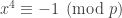if p ≡ 2 (mod 3), then $x^3 \equiv 1 \pmod p$ has a unique solution.

Problem 6. Prove that if p is an odd prime, then the congruence $x^4 \equiv -1 \pmod p$ has a solution if and only if p is 1 modulo 8.

Problem 7. (IMO 1998 shortlisted) Find all positive integers n such that there exists a positive integer m, satisfying

$(2^n - 1) | (m^2 + 9).$

Problem 8. Prove that if m, n are odd positive integers greater than 1, then $2^m - 1$ does not divide $3^n - 1$ . [ Note: this is where the link between quadratic residues and multiplicative order comes in handy. ]

Problem 9. (IMO 2008 Q3) Prove that there are infinitely many positive integers n such that n² + 1 has a prime factor which is greater than $2n + \sqrt{2n}$ .

Posted in Notes | Tagged intermediate, notes, number theory, quadratic residues | 3 Comments

Quadratic Residues – Part III

Posted on November 18, 2011 by limsup

Ok, here’s the third installation. Getting a little tired of repeatedly saying “a is/isn’t a square mod p“, we introduce a new notation.

Definition. Let p be an odd prime and a be an integer coprime to p. The Legendre symbol $(\frac a p)$ is given by:

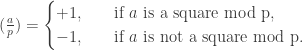
$(\frac a p) = \begin{cases} +1, \quad &\mbox{if } a \mbox{ is a square mod p},\\ -1,\quad &\mbox{if } a \mbox{ is not a square mod p}.\end{cases}$

For completeness, one also defines $(\frac a p) = 0$ if a is a multiple of p, but we won’t need this for now. From our previous post, we know the following:

$(\frac a p) \equiv a^{(p-1)/2} \pmod p$ ;
hence from property 1, $(\frac a p) (\frac b p) = ( \frac {ab} p )$ ;
for special values of a, we have $(\frac {-1} p) = (-1)^{(p-1)/2}$ and $(\frac 2 p) = (-1)^{(p^2-1)/8}$ .

From the multiplicative property (2), it thus suffices to consider $(\frac q p)$ for odd prime q ≠ p. This is where we’ll pull the next rabbit out of the hat (i.e. quote a result without proof).

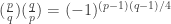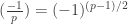
Quadratic Reciprocity Theorem. If p, q are distinct odd primes, then

$(\frac p q) (\frac q p) = (-1)^{(p-1)(q-1)/4}$ .

In other words, $(\frac p q)$ and $(\frac q p)$ are identical unless both p and q are congruent to 3 mod 4.

–

Example 1. Determine whether 31 is a square modulo 73.

Solution. We will repeatedly use the quadratic reciprocity rule:

$(\frac{31}{73}) (\frac{73}{31}) = +1$ since 73 is 1 mod 4, so $(\frac{31}{73}) = (\frac{73}{31}) = (\frac{11}{31})$ ;
$(\frac{11}{31}) (\frac{31}{11}) = -1$ since 31 ≡ 11 ≡ 3 (mod 4), so $(\frac{11}{31}) = -(\frac{31}{11}) = -(\frac {9}{11}) = -1$ since 9 is clearly a square mod 11.

Thus, 31 is not a square modulo 73. ♦

Example 2. Classify all odd primes p ≠ 3 such that 3 is a square modulo p.

Solution. Use the quadratic reciprocity: $(\frac 3 p) (\frac p 3) = (-1)^{(p-1)/2}$ . Since the RHS depends on p modulo 4, we need to consider p modulo 12. Thus, 3 is a square modulo p iff $(\frac p 3) = (-1)^{(p-1)/2}$ .

If $(\frac p 3) = (-1)^{(p-1)/2} = +1$ , then $p \equiv 1 \pmod 3$ and $p \equiv 1 \pmod 4$ , i.e. $p \equiv 1 \pmod {12}$ .
If $(\frac p 3) = (-1)^{(p-1)/2} = -1$ , then $p \equiv 2 \pmod 3$ and $p \equiv 3 \pmod 4$ , i.e. $p \equiv 11 \pmod {12}$ .

Thus 3 is a square mod p iff p ≡ ±1 (mod 12). ♦

Example 3. Classify all odd primes p ≠ 3 such that -3 is a square modulo p.

Solution. From example 1, we have $(\frac 3 p) = (\frac p 3) (-1)^{(p-1)/2}$ . Thus,

$(\frac {-3} p) = (\frac {-1} p) (\frac 3 p) = (-1)^{(p-1)/2}(\frac 3 p)=(\frac p 3)$ .

And -3 is a square mod p iff p ≡ 1 (mod 3). ♦

Coming up next: applying quadratic residues in conjunction with order of an element modulo n to solve IMO-type problems. The gist of the idea is this: suppose p is a prime and a be not divisible by p; let the (multiplicative) order of a modulo p be denoted d. We already know that d | (p-1). It turns out that a is a square modulo p if and only if $\frac {p-1} d$ is even.

To see why, just let g be a primitive root modulo p. And write $a \equiv g^r \pmod p$ . Now d is the smallest positive integer for which $a^d \equiv g^{rd} \equiv 1 \pmod p$ . Thus d is the smallest positive integer such that rd is a multiple of (p-1). A moment of thought will tell you that thus d = (p-1)/gcd(r, p-1) (prove it! just write g = gcd(r, p-1) and r = gu, (p-1) = gv where (u, v) = 1 … ).

Thus, our desired result follows from the fact that a is a square modulo p if and only if r is even. If you’re not sure why the fact is true, refer to part II of the notes. If you’re still confused, fret not, we will include some concrete examples in the next installation.

Posted in Notes | Tagged intermediate, legendre symbol, notes, number theory, quadratic residues | Leave a comment

Quadratic Residues – Part II

Posted on November 16, 2011 by limsup

Recall what we’re trying to do here: to show that if p > 2 is prime and a is not a square modulo p, then $a^{(p-1)/2} \equiv -1 \pmod p$ . As mentioned at the end of the previous part, we will need…

Primitive Roots

Again, let p > 2 be prime. For any a which is not divisible by p, recall that we have d = ord_p(a), which is the smallest positive integer d for which $a^d \equiv 1 \pmod p$ . We had proven earlier that d must divide p-1.

Definition : a primitive root is an element g mod p such that $ord_p(g) = p-1$ exactly.

In other words, among the elements $1, g, g^2, g^3, \dots, g^{p-2}$ (modulo p), only the first is equal to 1. In fact, we can say more: all these p-1 elements are distinct mod p! Indeed, if gⁱ ≡ g^j (mod p) for some 0 ≤ i < j ≤ p-2, then since g is coprime to p, we can do cancellation on both sides to obtain g^j-i ≡ 1 (mod p) where 0 < j-i ≤ p-2 which contradicts our assumption. So the p-1 elements $1, g, g^2, \dots, g^{p-2}$ are distinct and each is congruent to one of {1, 2, …, p-1}. In short:

If g is a primitive root, then the successive powers $1, g, g^2, \dots, g^{p-2}$ forms a permutation of {1, 2, …, p-1}.

E.g.

p = 7 : pick g = 3, then the successive powers of 3 give : $1, 3, 3^2 \equiv 2, 3^3 \equiv 6, 4, 5$ .
p = 13 : pick g = 2, then powers of 2 give 1, 2, 4, 8, 3, 6, 12, 11, 9, 5, 10, 7.

Now, we shall state a theorem without proof (with apology in advance … but it’s a very classical result and the reader should have no difficulty finding a book with proof).

Theorem. Every prime p has at least one primitive root.

Exercise 1: exactly how many primitive roots are there modulo p ?

Exercise 2: prove that if m is a positive integer not divisible by p-1, then $1^m + 2^m + \dots + (p-1)^m$ is a multiple of p.

–

Ok, now we’re ready to explain why $a^{(p-1)/2} \equiv -1 \pmod p$ for non-square a modulo p. Pick a primitive root g mod p. Since the powers of g (mod p) run through the entire set {1, 2, …, p-1} in some order, we have

$g^i \equiv a \pmod p$

for some i. We had already seen that $a^{(p-1)/2} \equiv \pm 1 \pmod p$ must hold, so it suffices to show $a^{(p-1)/2} \not\equiv +1 \pmod p$ . But if $a^{(p-1)/2} \equiv +1 \pmod p$ , then:

$g^{i(p-1)/2} \equiv +1 \pmod p$ .

Since the multiplicative order of g modulo p is exactly p-1, it just means that i(p-1)/2 is a multiple of p-1, i.e. i is a multiple of 2, so we write i = 2j. Thus, $a \equiv g^{2j}\equiv (g^j)^2 \pmod p$ is a square modulo p, which is a contradiction. ♦

Exercise 3 : prove that if p > 2 is prime, then (-1) is a square modulo p if and only if p is 1 modulo 4. [ Thanks to our theory of quadratic residues, this result is utterly trivial. ]

Exercise 4 : prove that if p > 2 is prime, then 2 is a square modulo p if and only if p ≡ ±1 (mod 8).

The last result is extremely important and not too easy, so we’ll guide you along with it. To read the hint, highlight the text starting from here … [ Hint : consider the elements 1, 2, … , (p-1)/2 modulo p. Upon multiplying them by 2, we obtain 2, 4, …, (p-1). Note that 2 × 4 × … × (p-3) × (p-1) ≡ (-1) × 2 × (-3) × 4 … . Now, multiply these (p-1)/2 numbers together, consider various cases modulo 8 and you’re done. ] … to here.

In the next chapter, we’ll introduce the Legendre symbol notation, an extremely handy notation for checking which numbers are squares mod p. Also, you’ll answer questions like “for what primes p is 3 a square mod p?”.

Posted in Notes | Tagged intermediate, notes, number theory, quadratic residues | Leave a comment

Quadratic Residues – Part I

Posted on November 15, 2011 by limsup

[ Background required : modular arithmetic. Seriously. ]

Warning: many of the proofs for theorems will be omitted in this set of notes, due to the length of the proofs.

The basic question we’re trying to answer in this series of notes is:

Let a be an integer mod m, so 0 ≤ a ≤ m-1. For which a, are there solutions to the congruence $x^2 \equiv a \pmod m$ ?

For some concrete examples:

m = 11 : then (±1)² ≡ 1, (±2)² ≡ 4, (±3)² ≡ 9, (±4)² ≡ 5, (±5)² ≡ 3, so the only squares modulo 11 are 0, 1, 3, 4, 5, 9;
m = 15 : then (±1)² ≡ 1, (±2)² ≡ 4, (±3)² ≡ 9, (±4)² ≡ 1, (±5)² ≡ 10, (±6)² ≡ 6, (±7)² ≡ 4, so the squares modulo 15 are 0, 1, 4, 6, 9, 10.

By Chinese Remainder Theorem, we know that solving a congruence modulo m is equivalent to solving it modulo prime powers, e. g. to solve something mod 135, it suffices to solve it mod 27 and mod 5, then piece the results together. In our above example of m = 15, notice that m = 10 is a square but m = 5 isn’t: because 5 modulo 3 = 2 is not a square mod 3.

In other words, we might as well assume m = p^r is a prime power. In fact, we will even assume m = p is an odd prime for now. The case of prime power is not significantly harder.

–

Let a be an integer which is not divisible by prime p > 2.

First, suppose a is a square mod p, i.e. we can find an x for which $x^2 \equiv a \pmod p$ . Since a is not divisible by p, neither is x. By Fermat’s little theorem, we get:

$1 \equiv x^{p-1} \equiv a^{\frac{p-1} 2} \pmod p$ .

In short, if a is a square, then $a^{(p-1)/2} \equiv 1 \pmod p$ .

On the other hand, what happens if a is not a square?

Let $x \equiv a^{(p-1)/2} \pmod p$ . Thanks to Fermat’s little theorem again, we have:

$x^2 \equiv a^{p-1} \equiv 1 \pmod p$ .

Thus, x²-1 is a multiple of p and so either x-1 or x+1 is a multiple of p, i.e. $x \equiv \pm 1 \pmod p$ . In conclusion, we have proven the following:

Let $m = p$ be an odd prime. For any a which is not divisible by p, let $x = a^{(p-1)/2}$ . Then

we always have x ≡ ±1 (mod p);

if a is a square mod p, then x ≡ 1 (mod p).

The big question is: what happens if a is not a square mod p??

It turns out, as the reader suspected, that if a is not a square mod p, then $a^{(p-1)/2} \equiv -1 \pmod p$ . E.g. take the case of p = 13 and a = 2, then we have $a^{(p-1)/2} = 2^6 = 64 \equiv -1 \pmod {13}$ .

To prove this in greater generality, we will need to introduce the concept of primitive roots in the next installation…

Posted in Notes | Tagged intermediate, notes, number theory, quadratic residues | Leave a comment

Number Theory Homework (2 Weeks)

Posted on November 14, 2011 by limsup

Homework problems for 5 Nov 2011:

Let a₁, a₂, … be a series recursively defined as follows: a₁ = 20, a₂ = 11, and for n ≥ 1, a_n+2 is the remainder when a_n+1 + a_n is divided by 100. What is the remainder when $a_1^2 + a_2^2 + \dots + a_{2011}^2$ is divided by 8?
(IMO 1962 Q1) Find the smallest positive integer with the following properties:

in decimal representation, its last digit is 6;
if we move this digit to the front of the number, we get 4 times the original number.

Find two 3-digit numbers (abc) and (def) such that upon placing them side-by-side, we get a 6-digit number (abcdef) satisfying : (abcdef) = ( (abc) + (def) )².
(a) A positive integer is written on the board. At each turn, we erase its unit digit and add 4 times that digit to the remaining number. Starting from 5²⁰¹¹, can we get 2011⁵ at some point? (b) Suppose instead, at each turn, we erase its unit digit and add 5 times that digit to the remaining number. Starting from 7²⁰¹¹, can we get 2011⁷ at some point?
Let a₁, a₂, … be a series recursively defined: a₀ = 1, a₁ = 3, and for n ≥ 0, a_n+2 = 6a_n+1 – a_n. Prove that for each n, either $\frac{a_n+1} 2$ or $\frac{a_n-1}2$ is a perfect square.

Homework problems for 12 Nov 2011:

Prove that if a, n are integers and n > 0, then whenever $a \equiv 1 \pmod n$ , we have $a^n \equiv 1 \pmod {n^2}$ .
Classify the solutions of $\frac 1 x + \frac 1 y = \frac 1 z$ , where x, y and z are positive integers.
Prove that if n =3^k, then n | (2ⁿ + 1). In particular, there are infinitely many n such that n | (2ⁿ + 1). Can you find an n with at least 2 distinct prime factors such that n | (2ⁿ + 1)?
(IMO 1971 shortlisted) Find all integer solutions to $x^2 + y^2 = (x-y)^3$ .
Suppose n is a positive integer such that n | (2ⁿ + 1). Prove that n = 1 or n is a multiple of 3.

[ Coming attractions : quadratic residues… stay tuned! 🙂 ]

Posted in Homework | Tagged basic, homework, number theory | 2 Comments

Thoughts on a Problem

Posted on November 8, 2011 by limsup

From time to time, I may post my experience in solving a specific problem including some wrong twists and turns I’ve taken, as well as the motivation for some rather cryptic constructions. Warning : since this post documents my thought process, it’s going to be extremely, perhaps even unnecessarily, verbose. Feedback will be appreciated, e.g. is this format too chatty and long-winded? Too many detours? Or…?

Today’s problem is Question A6 of Putnam 99.

The sequence a_n for n ≥ 1 is defined as follows: a₁ = 1, a₂ = 2, a₃ = 24 and for n ≥ 4, we have:

$a_n = \frac {6 a_{n-1}^2 a_{n-3} - 8 a_{n-1} a_{n-2}^2} {a_{n-2} a_{n-3}}.$

Prove that n divides a_n for any n ≥ 1.

Ready? Here goes.

The recurrence itself looks rather daunting. Now, let’s recall what kind of tools we have for solving recurrence relations: pretty much the most useful tool is that of solving linear recurrence relations. E.g. the Fibonacci sequence defined by $F_0 = 0, F_1 = 1$ and $F_{n+1} = F_n + F_{n-1}$ for n ≥ 1 has a closed form (known as Binet’s formula). Although I’ve not described in class how one can derive the closed form, it is a useful thing to keep in mind if you don’t know about it yet. There’s also the technique of power series, which deserves an entire lecture devoted to it, and from which one can derive some pretty cool sequences like the Catalan numbers.

But I’m digressing…

In any case, the above recurrence is clearly non-linear. And the irritating thing is that during competitions, one can’t use calculators and though it’s possible to get a₄ = 1344 by a bit of paperwork, getting the next term seems out of the question. In short, we can’t get enough terms to spot a pattern (within a competition anyway).

So the next thing we attempt to do can be quite a useful trick.

Attempt to Approximate the Size of a_n

Fine, if we can’t solve it yet, see if we can’t get a handle on how fast the sequence increases. From the first 4 terms, it seems clear the rate of increase is huge. Our next observation is that: the recurrence relation for a_n is a degree-3 relation divided by a degree-2 one, i.e. it is …. almost linear??

So let’s try our usual trick for linear recurrence relations and plug in $a_n \sim c\cdot \alpha^n$ for some fixed constant α. Let’s say this is a good approximation for $a_{n-3}, a_{n-2}, a_{n-1}$ , then plugging in gives…

$a_n \sim c \left[ \frac {6\alpha^{3n-5} - 8\alpha^{3n-5}} {\alpha^{2n-5}} \right] = -2c \alpha^n.$

Whoa, the next term is negative? A little unbelievable from what we could observe. This just means that our sequence is not increasing fast enough, i.e. our approximate is too low.

Ok, so let’s take $a_n \sim n!$ instead, dropping the constant since it’s clearly useless from our prior experience. This gives:

$a_n \sim \frac{6(n-1)!^2 (n-3)! - 8(n-1)!(n-2)!^2} {(n-2)! (n-3)!} = 6(n-1)! (n-1) - 8(n-1)! (n-3) = (n-1)! (-2n+18)$

No good! Eventually the terms will still become negative so our approximation still isn’t increasing fast enough. In fact, if you try $a_n \sim (kn)!$ for a fixed k, the recurrence eventually goes negative – but as k increases, that cross-over point becomes further and further away.

Ok, so maybe $(n^2)!$ ? We can’t handle that since $(n^2)! / (n-1)^2!$ is a disaster to manipulate.

Perhaps we can write $b_n = a_n / n!$ and rewrite the recurrence relation in terms of b_n‘s. We get (omitting the pesky details):

$b_n = \frac { 6 \left( \frac{n-1}n\right) b_{n-1}^2 b_{n-3} - 8 \left( \frac{n-2}n \right) b_{n-1} b_{n-2}^2} {b_{n-2} b_{n-3}}.$

This, by the way, can be a good trick : scaling down a term and writing the recurrence relation via another variable which is increasing at a more manageable rate.

In this case, this doesn’t help; we get a relation which is worse, and in fact, one can even argue that the two relations are “asymptotically identical” since as n becomes large, we can ignore (n-1)/n and (n-2)/n.

Ok, now what about the ratio between two successive terms : $b_n = a_n / a_{n-1}$ ? Upon writing this, we get our first breakthrough:

$b_n = \frac {a_n} {a_{n-1}} = \frac {6 a_{n-1} a_{n-3} - 8 a_{n-2}^2}{a_{n-2} a_{n-3}} = 6 \frac {a_{n-1}} {a_{n-2}} - 8 \frac {a_{n-2}} {a_{n-3}}$

i.e. $b_n = 6 b_{n-1} - 8 b_{n-2}$ , starting with b₂ = 2, b₃ = 12. A linear recurrence relation!! Let’s shift the indices so that b₀ = 2, b₁ = 12, thus giving us

$b_n = 4\cdot 4^n - 2\cdot 2^n = 4^{n+1} - 2^{n+1}.$

Shifting back the indices gives us $a_n = \prod_{i=2}^n (4^{n-1} - 2^{n-1})$ for n ≥ 2. The problem isn’t quite solved yet since we have yet to show n divides a_n, but it looks pretty close. To patch up the gaps:

if n=p is an odd prime, then by Fermat’s little theorem $4^{n-1} \equiv 1 \pmod n$ and $2^{n-1} \equiv 1 \pmod n$ so $4^{n-1} - 2^{n-1}$ is a multiple of n;
if n is divisible by p^r where p is an odd prime, then $4^{k(p-1)} - 2^{k(p-1)}$ is a multiple of p for k=1,2,…,r and r(p-1) clearly does not exceed n-1;
if n is divisible by 2^r then there’re far more than sufficient powers of 2 to go around.

Note: this article does not constitute a rigourous solution to the problem. The reader is advised to write up the proof properly. ◊

Posted in Thought | Tagged basic, intuition, number theory, thought | Leave a comment

Order of an Element Modulo m and Applications – Part II

Posted on November 6, 2011 by limsup

Having introduced the concept of the (multiplicative) order of a modulo m, let us use it to solve some problems.

Problem 1. Prove that if n > 1 is an integer, then n does not divide 2ⁿ – 1.

Proof. Since n > 1, we can pick the smallest prime factor p of n. Suppose, on the contrary, that n divides 2ⁿ – 1. Then p must also divide 2ⁿ – 1 so we have 2ⁿ ≡ 1 (mod p). On the other hand, since 2ⁿ – 1 is odd, p > 2 so we know by Fermat’s little theorem that 2^p^-1 ≡ 1 (mod p). Now if we let d be the multiplicative order of 2 modulo p, then d | n and d | (p-1). This shows that d is a factor of n which is even smaller than p. The only possibility is d = 1, i.e. 2¹ ≡ 1 (mod p) which is absurd. ♦

Problem 2. Prove that if m, n are positive integers with m odd, then 2^m – 1 and 2ⁿ + 1 are coprime.

Proof. Suppose they are not, so there is a prime p which divides both 2^m – 1 and 2ⁿ + 1. Note that p is odd. This means that: 2^m ≡ 1 (mod p) and 2ⁿ ≡ -1 (mod p). But the latter also implies 2²ⁿ ≡ 1 (mod p). Hence, if d is the multiplicative order of 2 modulo p, then d | m and d | 2n but d does not divide n. Thus, d divides 2n but not n, it must be 2k for some k | n. In particular, d is even, which contradicts the fact that d divides odd m. ♦

Problem 3. Prove that if k is a natural number and n = 2^k – 1 then k | φ(n).

Proof. This clearly holds for k = 1. For k > 1, let d = ord_n(2) – which is well-defined since n is odd. By Euler’s theorem, 2^φ(n) ≡ 1 (mod n) so we know that d divides φ(n). On the other hand, since n = 2^k – 1 it’s easy to compute d: the successive powers of 2 modulo n is given by: 1, 2, 2², … , 2^k-1, 2^k ≡ 1 (mod n). Since the first k terms are all < n, it is clear that d = k. Thus, k divides φ(n) as desired. ♦

Here are more problems which can be solved by skilfully applying the concept of order.

Problem 4. Prove that if p is prime, then p^p – 1 has a prime factor which is congruent to 1 mod p.

Problem 5. Prove that if n is even, then any divisor of n⁴ + 1 is congruent to 1 mod 8. Can you generalise the result?

Problem 6. Prove that if n is even and not a multiple of 3, then any divisor of n² + 3 is congruent to 1 mod 3. [ PS. The solution to this problem can be somewhat simplified with quadratic reciprocity, something which I will hopefully cover at a later date. ]

Problem 7. [ IMO 1989 Shortlisted ] Let m > 1 be an integer. Find the smallest positive integer n such that 2¹⁹⁸⁹ divides mⁿ – 1.

Posted in Notes | Tagged intermediate, notes, number theory | 2 Comments