Here is the main problem we are trying to solve today.
Word Problem
Given a word  let us consider
  disjoint subwords of
  which are weakly increasing. For example if
  , then we can pick two or three disjoint subwords as follows:

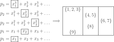
For each  , we wish to compute
  , the maximum length sums of disjoint weakly increasing subwords. In our example,
  However,
  since we can add the second ‘5’ to the circles, thus using up 8 numbers in the word. It turns out we do have
  although this is not obvious at the moment.
There is at least one case where computing is trivial.
Proposition 1. If  for some SSYT
  of shape
  , then for each we have:

Proof
Indeed if has rows  , then
  and the words
  are disjoint weakly increasing words of the required length sum. Hence
Conversely, if  are disjoint weakly increasing subwords of
  , the numbers in each
  are from different columns of . So in each column of
  at most entries are used among the and the length sum of is at most
  ♦
♦

General Solution
The good news is, every case can be reduced to the SSYT case. Indeed, given any word  we can write for some skew SSYT
  Now we perform sliding operations to turn into an SSYT
  By the next result,
  for all k, so we can revert to the above special case.
Proposition 2. If  are Knuth-equivalent words, then
Proof
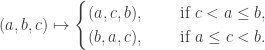
We may assume  is obtained from by rule R1 or R2. Let us consider each case.
R1: in we have a consecutive triplet  with
with  ; we swap
  and
and  to get
  In most instances, disjoint weakly increasing subwords of will remain so in and vice versa. The only problem is when a subword of contains
  , say
, say  If no subword contains
  we can replace with
  and the resulting word is still weakly increasing. If not, we swap the heads:

which are still weakly increasing.
R2: similarly, in we have a consecutive triplet with  ; swap
  and to get The critical case is now as follows:

This completes the proof. ♦
Summary
Thus we have:
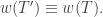
Algorithm. To compute , write for a skew SSYT , perform the sliding algorithm to turn into an SSYT  of shape
  Now we have:
 for all
E.g. in our initial example of (1, 1, 5, 4, 2, 5, 4, 6, 7), first write it as a word of some skew SSYT, then perform sliding to turn it into an SSYT.

It follows that  ,
,  and
and  .
.
Question to Ponder
Besides computing , what is an efficient way to compute explicit disjoint subwords with the desired length sum?
Uniqueness of SSYT for Word
We need the following lemma for our theorem later.
Lemma. If  and
and  (resp.
  ) is obtained from (resp. ) by removing the largest element, then
  The same holds for the smallest element.
Here, if the maximal element of occurs more than once, the rightmost occurrence is taken to be the largest. Similarly, the leftmost occurrence of the minimal element is the smallest.
Proof
We may assume is obtained from by R1 or R2, i.e. by replacing a consecutive triplet:
If none of  is maximal, we are done. Otherwise, in both cases, is maximal; after removing it, we get
  in and
In the case the smallest element is removed, in the first case we remove and obtain  in both and In the second case, we remove and obtain
  in both and ♦
Now we have enough tools to prove the following result we claimed earlier.
Theorem. For any word there is a unique SSYT such that 
We call this the rectification of the word  For a skew SSYT
  the rectification of
  is also called the rectification of
Proof
Existence of was proven earlier; we now prove uniqueness, i.e. for any SSYT 

By proposition 2, the shape of satisfies

so and have the same shape. Now we proceed by induction on  ; when
  we clearly have
Suppose  and
and  is the largest element in and
  if this occurs more than once, we take the rightmost occurrence. Note that must lie in a corner square of and Removing it thus gives us SSYT
  and
and  By the above lemma, we have

Since has one less square than , by induction hypothesis  And since and have the same shape, we have ♦
Summary
There is a bijection:

The bijection is preserved when we drop the maximum or minimum element in either case. Clearly concatenation preserves Knuth-equivalence:

since any sequence of R1’s and R2’s performed on  can be done on
  Thus this gives an associative product operation on the set of SSYT: given let
  be the rectification of
  This motivates the product operation we defined earlier.


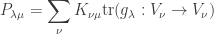
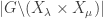
![[g_\lambda]](https://s0.wp.com/latex.php?latex=%5Bg_%5Clambda%5D&bg=ffffff&fg=333333&s=0&c=20201002)


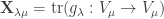
![U_\mu = \mathbb{C}[X_\mu].](https://s0.wp.com/latex.php?latex=U_%5Cmu+%3D+%5Cmathbb%7BC%7D%5BX_%5Cmu%5D.&bg=ffffff&fg=333333&s=0&c=20201002)
acts on finite set
, then the trace of
is:
, the number of fixed points of
in

![\mathbb{C}[X]](https://s0.wp.com/latex.php?latex=%5Cmathbb%7BC%7D%5BX%5D&bg=ffffff&fg=333333&s=0&c=20201002)


be the trace of
on
as a sum of monomials, we get:


![[d] = \coprod_i A_i,](https://s0.wp.com/latex.php?latex=%5Bd%5D+%3D+%5Ccoprod_i+A_i%2C&bg=ffffff&fg=333333&s=0&c=20201002)


is the order of the centralizer of any


 corresponds to on the RHS.
 and
and  where
where  Multiplication gives
  where
where  is the partition obtained by sorting
  Next, we use the following standard result.
 and let
  be its stabiliser. Then:
![\mathbb{C}[X] \cong \text{Ind}_H^G \mathbb{C},](https://s0.wp.com/latex.php?latex=%5Cmathbb%7BC%7D%5BX%5D+%5Ccong+%5Ctext%7BInd%7D_H%5EG+%5Cmathbb%7BC%7D%2C&bg=ffffff&fg=333333&s=0&c=20201002)
 induced to
![\mathbb{C}[G] \otimes_{\mathbb{C}[H]} \mathbb{C}](https://s0.wp.com/latex.php?latex=%5Cmathbb%7BC%7D%5BG%5D+%5Cotimes_%7B%5Cmathbb%7BC%7D%5BH%5D%7D+%5Cmathbb%7BC%7D&bg=ffffff&fg=333333&s=0&c=20201002) by definition. Now we map
by definition. Now we map  on the LHS to
  on the RHS. Now:
![U_\lambda = \mathbb{C}[X_\lambda]](https://s0.wp.com/latex.php?latex=U_%5Clambda+%3D+%5Cmathbb%7BC%7D%5BX_%5Clambda%5D&bg=ffffff&fg=333333&s=0&c=20201002) is isomorphic to
is isomorphic to  where
where  and
and  Clearly
  so we have:

 corresponds to:
 acts on
  via
via 
 are
are  -algebras,
  are subalgebras, and
  are
are  -modules respectively. Then
![B=\mathbb{C}[G],\quad B' = \mathbb{C}[G'],\quad A=\mathbb{C}[H],\quad A'=\mathbb{C}[H']](https://s0.wp.com/latex.php?latex=B%3D%5Cmathbb%7BC%7D%5BG%5D%2C%5Cquad+B%27+%3D+%5Cmathbb%7BC%7D%5BG%27%5D%2C%5Cquad+A%3D%5Cmathbb%7BC%7D%5BH%5D%2C%5Cquad+A%27%3D%5Cmathbb%7BC%7D%5BH%27%5D&bg=ffffff&fg=333333&s=0&c=20201002)
 and
and  . Since
 ![\mathbb{C}[G\times G'] \cong \mathbb{C}[G]\otimes \mathbb{C}[G']](https://s0.wp.com/latex.php?latex=%5Cmathbb%7BC%7D%5BG%5Ctimes+G%27%5D+%5Ccong+%5Cmathbb%7BC%7D%5BG%5D%5Cotimes+%5Cmathbb%7BC%7D%5BG%27%5D&bg=ffffff&fg=333333&s=0&c=20201002) as
as 
 So we have:
 as desired. ♦
 and the set of virtual representations of all

 corresponds to
  By
By  where
where 

 and
and  ,
,
 where the sum is over all partitions
  by removing one box.
 and
and  as a direct sums of irreps where
 and hence any field of characteristic 0. For convenience we will fix
  .
. over
over  if
if  is a group homomorphism, we can twist
  as follows:
 for the twist; this gives an action on the set of all irreducible representations of G. Note that
  so the dimension of V is invariant among the equivalence classes of twists.
 .
. we let
  be the alternating character, i.e.
  Now we consider the modules
 ![U_\lambda \otimes \chi = \mathbb{C}[X_\lambda] \otimes \chi.](https://s0.wp.com/latex.php?latex=U_%5Clambda+%5Cotimes+%5Cchi+%3D+%5Cmathbb%7BC%7D%5BX_%5Clambda%5D+%5Cotimes+%5Cchi.&bg=ffffff&fg=333333&s=0&c=20201002)
![\left< U_\mu, U_\lambda \otimes \chi\right> = \dim_{\mathbb{C}} \text{Hom}_{\mathbb{C}[G]}(U_\mu, U_\lambda \otimes\chi)?](https://s0.wp.com/latex.php?latex=%5Cleft%3C+U_%5Cmu%2C+U_%5Clambda+%5Cotimes+%5Cchi%5Cright%3E+%3D+%5Cdim_%7B%5Cmathbb%7BC%7D%7D+%5Ctext%7BHom%7D_%7B%5Cmathbb%7BC%7D%5BG%5D%7D%28U_%5Cmu%2C+U_%5Clambda+%5Cotimes%5Cchi%29%3F&bg=ffffff&fg=333333&s=0&c=20201002)
 is the same as
  though the action has a twist. Recall that, as
 ![\text{Hom}_\mathbb{C}(U_\mu, U_\lambda \otimes \chi) \cong \mathbb{C}[X_\mu] \otimes \mathbb{C}[X_\lambda] \otimes \chi\cong \mathbb{C}[X_\mu \times X_\lambda] \otimes \chi](https://s0.wp.com/latex.php?latex=%5Ctext%7BHom%7D_%5Cmathbb%7BC%7D%28U_%5Cmu%2C+U_%5Clambda+%5Cotimes+%5Cchi%29+%5Ccong+%5Cmathbb%7BC%7D%5BX_%5Cmu%5D+%5Cotimes+%5Cmathbb%7BC%7D%5BX_%5Clambda%5D+%5Cotimes+%5Cchi%5Ccong+%5Cmathbb%7BC%7D%5BX_%5Cmu+%5Ctimes+X_%5Clambda%5D+%5Cotimes+%5Cchi&bg=ffffff&fg=333333&s=0&c=20201002)
 on the RHS is a linear combination of elements
  Let us unwind the definition for
 ![[d] = A_1 \coprod \ldots \coprod A_l = B_1 \coprod \ldots \coprod B_m, \qquad |A_i| = \mu_i, |B_j| = \lambda_j](https://s0.wp.com/latex.php?latex=%5Bd%5D+%3D+A_1+%5Ccoprod+%5Cldots+%5Ccoprod+A_l+%3D+B_1+%5Ccoprod+%5Cldots+%5Ccoprod+B_m%2C+%5Cqquad+%7CA_i%7C+%3D+%5Cmu_i%2C+%7CB_j%7C+%3D+%5Clambda_j&bg=ffffff&fg=333333&s=0&c=20201002)
 takes it to
 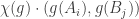 . Now if any
  has more than one element, then the transposition
  which swaps them would flip the sign while leaving
  ,
,  . Thus we have shown:
 for some
  , then the coefficient of
  in
in  for all
  so we get
![[3] = \overbrace{\{2,3\}}^{A_1} \cup \overbrace{\{1\}}^{B_1} = \overbrace{ \{1,3\} }^{A_2} \cup \overbrace{\{2\}}^{B_2} = \overbrace{ \{1,2\} }^{A_3} \cup \overbrace{ \{3\}}^{B_3}.](https://s0.wp.com/latex.php?latex=%5B3%5D+%3D+%5Coverbrace%7B%5C%7B2%2C3%5C%7D%7D%5E%7BA_1%7D+%5Ccup+%5Coverbrace%7B%5C%7B1%5C%7D%7D%5E%7BB_1%7D+%3D+%5Coverbrace%7B+%5C%7B1%2C3%5C%7D+%7D%5E%7BA_2%7D+%5Ccup+%5Coverbrace%7B%5C%7B2%5C%7D%7D%5E%7BB_2%7D+%3D+%5Coverbrace%7B+%5C%7B1%2C2%5C%7D+%7D%5E%7BA_3%7D+%5Ccup+%5Coverbrace%7B+%5C%7B3%5C%7D%7D%5E%7BB_3%7D.&bg=ffffff&fg=333333&s=0&c=20201002)
 has 9 elements
  for
for  . Any invariant element in
 ![\mathbb{C}[X_\mu \times X_\lambda]\otimes \chi](https://s0.wp.com/latex.php?latex=%5Cmathbb%7BC%7D%5BX_%5Cmu+%5Ctimes+X_%5Clambda%5D%5Cotimes+%5Cchi&bg=ffffff&fg=333333&s=0&c=20201002) must be a multiple of:
must be a multiple of: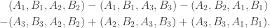
![\left<U_\mu, U_\lambda\otimes \chi\right> = \text{Hom}_{\mathbb{C}[G]}(U_\mu, U_\lambda \otimes \chi) = N_{\lambda\mu},](https://s0.wp.com/latex.php?latex=%5Cleft%3CU_%5Cmu%2C+U_%5Clambda%5Cotimes+%5Cchi%5Cright%3E+%3D+%5Ctext%7BHom%7D_%7B%5Cmathbb%7BC%7D%5BG%5D%7D%28U_%5Cmu%2C+U_%5Clambda+%5Cotimes+%5Cchi%29+%3D+N_%7B%5Clambda%5Cmu%7D%2C&bg=ffffff&fg=333333&s=0&c=20201002)
 such that
  and
and 
 satisfies:
 Writing
  we get:
 then writing in matrix form gives
  Hence
Hence  and we have
  Thus:
Thus:
 is invertible we have proven:
 if and only if
  is
is 
 which maps
  corresponds to
  This gives an algebraic interpretation for
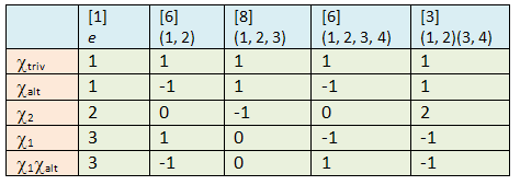
 . We get 3 partitions:
  ,
,  and
and  Let us compute
  for all
  From the
 ,
,  is absolutely irreducible (i.e. irreducible even over the algebraic closure of K). Since
 and
and  contains exactly one copy of
  Thus we write
 does not contain
  . Hence
 , we obtain:
 so
so  is absolutely irreducible. Since
  ,
,  contains two copies of
  Thus we write:
 does not contain

 Indeed, the representations
 ![U_\lambda := K[X_\lambda]](https://s0.wp.com/latex.php?latex=U_%5Clambda+%3A%3D+K%5BX_%5Clambda%5D&bg=ffffff&fg=333333&s=0&c=20201002) satisfy:
satisfy:
 satisfies
  where
where  is the number of SSYT of shape
  for all
  , then
  and so
  lexicographically.
 is a finite partially ordered set and
  is a collection of representations. And suppose there are non-negative integers
  satisfying
 defined over K such that:
 ; then
 is absolutely irreducible. The number of copies of
  contained in each
  is:
is:
 where
where  does not contain
  This then gives us:
 with
with  satisfy the given conditions and we may proceed recursively with this reduced set. ♦
 and the representations
  we get:
 of
of 
 such that:
 is the number of SYT of shape
  where
where  Now
Now  and
and which we had proven earlier with the
  be the character for the irrep
 then
then  and the Hall inner product
  corresponds to
 ![(V, W) \mapsto \dim_K \text{Hom}_{K[G]}(V, W).](https://s0.wp.com/latex.php?latex=%28V%2C+W%29+%5Cmapsto+%5Cdim_K+%5Ctext%7BHom%7D_%7BK%5BG%5D%7D%28V%2C+W%29.&bg=ffffff&fg=333333&s=0&c=20201002)
 and the group of virtual characters of
  where
where  are group characters. The set of virtual characters of a finite group G forms a
  , the space of symmetric polynomials of degree d with rational coefficients;
 .
.![g: [d] \to [d].](https://s0.wp.com/latex.php?latex=g%3A+%5Bd%5D+%5Cto+%5Bd%5D.&bg=ffffff&fg=333333&s=0&c=20201002) From here on, we shall look at the representations of
From here on, we shall look at the representations of  be the set of partitions of
 ![[d]](https://s0.wp.com/latex.php?latex=%5Bd%5D&bg=ffffff&fg=333333&s=0&c=20201002) into disjoint subsets
into disjoint subsets  such that
  for each
  The group
 , the partitioning is considered different when we swap
  and
and  For example if d = 4 and
  , then

![K[G]](https://s0.wp.com/latex.php?latex=K%5BG%5D&bg=ffffff&fg=333333&s=0&c=20201002) -module for any field K. Two special cases are of interest.
-module for any field K. Two special cases are of interest. : X has a single element so
  : X is just the set of permutations of [d] so
  ,
, ![[d].](https://s0.wp.com/latex.php?latex=%5Bd%5D.&bg=ffffff&fg=333333&s=0&c=20201002)
![K[X]^\vee \cong K[X]](https://s0.wp.com/latex.php?latex=K%5BX%5D%5E%5Cvee+%5Ccong+K%5BX%5D&bg=ffffff&fg=333333&s=0&c=20201002) (i.e.
(i.e. ![K[X]](https://s0.wp.com/latex.php?latex=K%5BX%5D&bg=ffffff&fg=333333&s=0&c=20201002) is isomorphic to its dual);
is isomorphic to its dual);![K[X] \otimes_K K[Y] \cong K[X\times Y]](https://s0.wp.com/latex.php?latex=K%5BX%5D+%5Cotimes_K+K%5BY%5D+%5Ccong+K%5BX%5Ctimes+Y%5D&bg=ffffff&fg=333333&s=0&c=20201002) ;
;![\text{Hom}_K(K[X], K[Y]) \cong K[X\times Y]](https://s0.wp.com/latex.php?latex=%5Ctext%7BHom%7D_K%28K%5BX%5D%2C+K%5BY%5D%29+%5Ccong+K%5BX%5Ctimes+Y%5D&bg=ffffff&fg=333333&s=0&c=20201002) ;
;![K[X]^G = \{v\in K[X] : \forall g\in G, gv = v\}](https://s0.wp.com/latex.php?latex=K%5BX%5D%5EG+%3D+%5C%7Bv%5Cin+K%5BX%5D+%3A+%5Cforall+g%5Cin+G%2C+gv+%3D+v%5C%7D&bg=ffffff&fg=333333&s=0&c=20201002) has dimension
has dimension  , the number of orbits of X.
![K[X] \times K[X] \to K](https://s0.wp.com/latex.php?latex=K%5BX%5D+%5Ctimes+K%5BX%5D+%5Cto+K&bg=ffffff&fg=333333&s=0&c=20201002) induced linearly from the map:
induced linearly from the map:
![K[X] \to K[X]^\vee](https://s0.wp.com/latex.php?latex=K%5BX%5D+%5Cto+K%5BX%5D%5E%5Cvee&bg=ffffff&fg=333333&s=0&c=20201002) of vector spaces. It is also G-equivariant since the bilinear map is G-equivariant, which proves the first statement.
of vector spaces. It is also G-equivariant since the bilinear map is G-equivariant, which proves the first statement.![K[X]\otimes_K K[Y] \cong K[X \times Y]](https://s0.wp.com/latex.php?latex=K%5BX%5D%5Cotimes_K+K%5BY%5D+%5Ccong+K%5BX+%5Ctimes+Y%5D&bg=ffffff&fg=333333&s=0&c=20201002) as vector spaces, taking
as vector spaces, taking  One easily checks that it is G-equivariant.
 for any K[G]-modules V and W. Thus:
![\text{Hom}_K(K[X], K[Y]) \cong K[X]^\vee \otimes_K K[Y] \cong K[X] \otimes_K K[Y] \cong K[X\times Y].](https://s0.wp.com/latex.php?latex=%5Ctext%7BHom%7D_K%28K%5BX%5D%2C+K%5BY%5D%29+%5Ccong+K%5BX%5D%5E%5Cvee+%5Cotimes_K+K%5BY%5D+%5Ccong+K%5BX%5D+%5Cotimes_K+K%5BY%5D+%5Ccong+K%5BX%5Ctimes+Y%5D.&bg=ffffff&fg=333333&s=0&c=20201002)
![\sum_{x\in X} c_x x\in K[X]](https://s0.wp.com/latex.php?latex=%5Csum_%7Bx%5Cin+X%7D+c_x+x%5Cin+K%5BX%5D&bg=ffffff&fg=333333&s=0&c=20201002) is invariant under every
is invariant under every  for all
  Thus
Thus  is constant when
  runs through an orbit. ♦
 what is the following value:
![\displaystyle \left<U_\mu, U_\lambda\right>_G = \dim_L\text{Hom}_{L[G]}(L[X_\mu], L[X_\lambda])](https://s0.wp.com/latex.php?latex=%5Cdisplaystyle+%5Cleft%3CU_%5Cmu%2C+U_%5Clambda%5Cright%3E_G+%3D+%5Cdim_L%5Ctext%7BHom%7D_%7BL%5BG%5D%7D%28L%5BX_%5Cmu%5D%2C+L%5BX_%5Clambda%5D%29&bg=ffffff&fg=333333&s=0&c=20201002)
 is the algebraic closure of
  ?
? to simplify matters, in which case L = K and when we mention “absolutely irreducible”, just replace it with “irreducible”.
![\text{Hom}_{K[G]} (K[X_\mu], K[X_\lambda]) =\text{Hom}_K (K[X_\mu], K[X_\lambda])^G \cong K[X_\lambda \times X_\mu]^G](https://s0.wp.com/latex.php?latex=%5Ctext%7BHom%7D_%7BK%5BG%5D%7D+%28K%5BX_%5Cmu%5D%2C+K%5BX_%5Clambda%5D%29+%3D%5Ctext%7BHom%7D_K+%28K%5BX_%5Cmu%5D%2C+K%5BX_%5Clambda%5D%29%5EG+%5Ccong+K%5BX_%5Clambda+%5Ctimes+X_%5Cmu%5D%5EG&bg=ffffff&fg=333333&s=0&c=20201002)
 . Writing
  and
and  let us pick
  and
and  Then the orbit of the pair
  satisfies:
 and
and  are partitions of [d] satisfying:
 so the pairs


 of shape
  is the number of skew SSYT of shape
  whose rectification is
  Since this number is independent of our choice of
  we take the most natural one.
 -th row comprises of all
  For example, the following is a canonical SSYT of shape (5, 4, 3).
 is the number of skew SSYT of shape
 is a reverse lattice word if, for each
  , the substring
  has at least as many 1’s as it has 2’s, at least as many 2’s as it has 3’s, etc.
 , for each
  in
in  then replace
  to form
  the four words on the left are OK if and only if the four words on the right are OK.
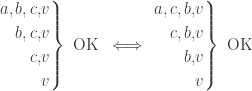

 where
where  and
and  To express
  Thus:
Thus:
 for various

 as a linear sum of Schur polynomials. For each partition

 then define a pair of SSYT of the same shape via:
 ,
, and
and  is obtained from
  by appending
  so that it has the same shape as
 .
. and since
  we get:
 is Knuth-equivalent to the word
  In other words,
  is the rectification of
  of the same shape gives us the two-row matrix
  Now let
  and
and  ;
; , let
, let  , and
, and  to it, and filling in
 is a skew SSYT whose rectification is
 and the initial SSYT
  . This gives:
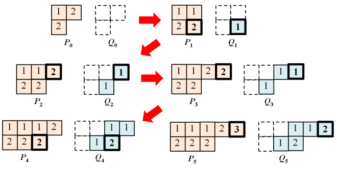
 is
is  , which is consistent with our claim.
 which are strictly smaller than all


 By the
 satisfies
 some order of
 On the RHS, this gives some order of
  is the rectification of that same order of
  and we are done. ♦
 be partitions. Suppose
  is an SSYT of shape
  respectively, such that

 is the rectification of the skew SSYT obtained by putting
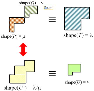
 for all
  be of shapes
  respectively such that
  The RSK correspondence for
  gives us a two-row matrix:
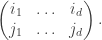
 be the SSYT obtained from
  and
and  in the new empty boxes. By construction we have
  so
so  By theorem 1, the rectification of
  Let
Let  of shape
 corresponds via RSK to a two-row matrix:
 are from
  of shape
  The remaining
  columns correspond to a pair
  which gives
  as desired. ♦
 is dependent only on
  , and independent of the choice of
  .
.  over all skew SSYT
 over all partitions
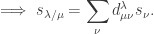
 and our
  is precisely the
  Given a skew SSYT
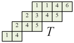
 elements of the sequence diagonally: 1st row and
  -th square etc.

 in the SSYT with
 and we get
  . Break this down into a series of steps:
 , we switch
 to the beginning of the row, we break it down as follows:
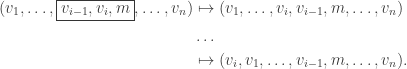
 , we switch
 . Applying R1 and R2 gives:
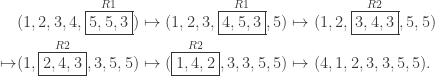
 or
or  : no change;
 by R1;
 : switch to
  by R2;
 : switch to
  : switch to
  if we can obtain one from the other via the above 4 operations.
 .
.
 for
for 
 for
for  etc. First consider the case
  i.e. we need to show
 into
into  Since
Since  this bumps out
  and we transform
  to
to 
 into this row then bumps out
  and we obtain
  Moving on, we eventually obtain
  as desired.
 Write
Write  and
and  so that
  and
and  We need to show
 into the row
  bumps off
  which gives
  Thus the LHS is equivalent to
  By induction hypothesis for
  this is equivalent to
 to give
  Hence the RHS is equivalent to
  for some skew SSYT
  by a horizontal or vertical line (where
 so the result is trivial. Now suppose we have a vertical cut as follows.
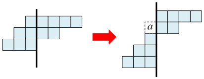
 ♦
♦ and
and  then
then  where
where  and
and 

 of
of 


