Polynomials and Representations XXXI | Mathematics and Such

Polynomials and Representations XXXI

Posted on June 19, 2016 by limsup

K-Representations and G-Representations

As mentioned at the end of the previous article, we shall attempt to construct analytic representations of $G = GL_n\mathbb{C}$ from continuous representations of $K = U_n.$

Let $\rho : K \to GL(V)$ . Consider $\rho|_S$ , where $S$ is the group of diagonal matrices in K so

$S = \left\{\begin{pmatrix} e^{i\theta_1} & 0 & \ldots & 0 \\ 0 & e^{i\theta_2} & \ldots & 0\\ \vdots & \vdots & \ddots &\vdots\\ 0 & 0 & \ldots & e^{i\theta_n}\end{pmatrix} : \theta_1, \ldots, \theta_n \in \mathbb{R}\right\} \cong (\mathbb R/\mathbb Z)^n$

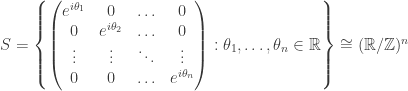
as a topological group. From our study of representations of the n-torus, we know that $\rho|_S$ is a direct sum of 1-dimensional irreps of the form:

$\rho_{\mathbf a} = \rho_{a_1, \ldots, a_n} : S \to \mathbb C^*, \quad \begin{pmatrix}x_1 & \ldots & 0 \\ \vdots & \ddots & \vdots \\ 0 & \ldots & x_n \end{pmatrix} \mapsto x_1^{a_1} \ldots x_n^{a_n},$

where $\mathbf a = (a_1, \ldots, a_n) \in \mathbb Z^n$ . E.g. if $\mathbf a = \mathbf 0$ then the representation is trivial; if $\mathbf a = (1,\ldots, 1),$ the representation is obtained by taking the determinant.

Hence, the character of $\rho|_S$ is a Laurent polynomial with non-negative integer coefficients, i.e.

$\chi(\rho|_S) \in \mathbb{Z}[x_1, \ldots, x_n, x_1^{-1}, \ldots, x_n^{-1}].$

Definition. For a continuous finite-dimensional representation $\rho :K \to GL (V)$ , we will write $\psi_V$ for $\chi(\rho|_S)$ expressed as a Laurent polynomial in $x_1, \ldots x_n$ .

The same holds for a complex analytic representation of G.

Examples

If $\rho: G \to GL (\mathbb C^n)$ is the identity map, its Laurent polynomial is $x_1 + x_2 + \ldots + x_n.$
For $\det : G\to \mathbb C^*$ , its Laurent polynomial is $x_1 x_2 \ldots x_n.$

The following are clear for any continuous representations V, W of K.

$\begin{aligned} \psi_{V\oplus W} &= \psi_V + \psi_W \\ \psi_{V\otimes W} &= \psi_V \cdot \psi_W\\ \psi_{V} &= \psi_W + \psi_{V/W} \text{ if } W\subseteq V \\ \psi_{V^\vee}(x_1, \ldots, x_n) &= \psi_V(x_1^{-1}, \ldots, x_n^{-1}).\end{aligned}$

In summary, so far we have the following:

representations_correspondences

blue-lin

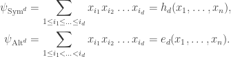
Main Examples: Sym and Alt

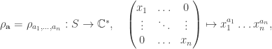
For any vector space V, the group $S_d$ acts on $V^{\otimes d}$ by permuting the components. We denote:

$\begin{aligned} \text{Sym}^d V &:= \{ v \in V^{\otimes d} : w(v) = v \text{ for each } w\in S_d\},\\ \text{Alt}^d V &:= \{ v \in V^{\otimes d} : w(v) = \chi(w)v \text{ for each } w\in S_d\}\end{aligned}$

where $\chi(w)$ is the sign of w. Let $e_1, \ldots, e_n$ be a fixed basis of V. The case d=2 is quite easy to describe for the above spaces, for we can just take the following bases:

$\text{Sym}^2 V : \{ e_i \otimes e_j + e_j \otimes e_i : 1 \le i \le j \le n\}$ ;
$\text{Alt}^2 V : \{ e_i \otimes e_j - e_j \otimes e_i : 1 \le i < j \le n\}$ .

Denote these two types of elements by $e_i e_j$ and $e_i \wedge e_j$ respectively, so that $e_i e_j = e_j e_i$ and $e_i \wedge e_j = -e_j \wedge e_i.$ Note that $V\otimes V \cong \text{Sym}^2 V \oplus\text{Alt}^2 V$ ; this is not true for higher values of d.

Similarly, in general, we can pick the following as bases:

$\text{Sym}^d V : \{ e_{i_1} \ldots e_{i_d} : 1 \le i_1 \le \ldots \le i_d \le n\}$ ;
$\text{Alt}^d V : \{ e_{i_1} \wedge \ldots \wedge e_{i_d}: 1 \le i_1 < \ldots < i_d \le n\}$ .

where the components commute in Sym and anticommute in Alt (e.g. $e_1 \wedge e_2 \wedge e_4 = - e_2 \wedge e_1 \wedge e_4 = e_2 \wedge e_4 \wedge e_1$ ).

Now suppose $V = \mathbb{C}^n$ and $G = GL_n\mathbb{C}$ acts on it; G and $S_d$ act on $V^{\otimes d}$ in the following manner:

$\begin{aligned} g\in G &\implies g(v_1 \otimes \ldots \otimes v_d) = g(v_1) \otimes \ldots \otimes g(v_d), \\ w\in S_d &\implies w(v_1 \otimes \ldots \otimes v_d) = v_{w^{-1}(1)} \otimes \ldots \otimes v_{w^{-1}(d)}.\end{aligned}$

These two actions commute, from which one easily shows that $\text{Sym}^d V$ and $\text{Alt}^d V$ are G-invariant subspaces of $V^{\otimes d}$ .

Example

Suppose we have $g = \begin{pmatrix} 2 & -1\\ 1 & 3\end{pmatrix}$ acting on $\text{Sym}^3 \mathbb{C}^2$ . This takes:

$e_1^2 e_2 \mapsto (2e_1 - e_2)^2 (e_1 + 3e_2) = 4e_1^3 + 8e_1^2 e_2 - 11e_1 e_2^2 + 3e_2^3.$

To compute the Laurent polynomials of these spaces, we let the diagonal matrix $D(x_1, \ldots, x_n)$ act on them, giving:

$\begin{aligned} e_{i_1} e_{i_2} \ldots e_{i_d} &\mapsto (x_{i_1} x_{i_2} \ldots x_{i_d}) e_{i_1} e_{i_2} \ldots e_{i_d},\\ e_{i_1} \wedge \ldots \wedge e_{i_d}& \mapsto (x_{i_1} x_{i_2}\ldots x_{i_d}) e_{i_1} \wedge \ldots \wedge e_{i_d}.\end{aligned}$

Hence we have:

$\displaystyle\begin{aligned} \psi_{\text{Sym}^d} &= \sum_{1\le i_1 \le \ldots \le i_d} x_{i_1} x_{i_2} \ldots x_{i_d} = h_d(x_1, \ldots, x_n),\\ \psi_{\text{Alt}^d} &= \sum_{1 \le i_1 < \ldots < i_d} x_{i_1} x_{i_2} \ldots x_{i_d} = e_d(x_1, \ldots, x_n).\end{aligned}$

blue-lin

Some Lemmas

Lemma 1. For a representation V of K, the Laurent polynomial $\psi_V$ is symmetric.

Proof

For any $w\in S_n$ , take the corresponding permutation matrix $M\in K$ ; we have:

$\displaystyle M\cdot \begin{pmatrix} x_1 & \ldots & 0 \\ \vdots & \ddots & \vdots \\0 & \ldots & x_n \end{pmatrix}\cdot M^{-1} = \begin{pmatrix}x_{w(1)} & \ldots & 0 \\ \vdots & \ddots & \vdots \\0 & \ldots & x_{w(n)}\end{pmatrix}.$

Thus $\psi_V(x_1, \ldots, x_n) = \psi_V(x_{w(1)}, \ldots, x_{w(n)})$ for any $w\in S_n.$ ♦

Lemma 2. Given K-representations V, W, if $\psi_{V} = \psi_{W}$ , then $V\cong W.$

Hence by the previous article, the same holds for analytic G-representations V, W.

Proof

Any $M\in K$ , being unitary, is diagonalizable by a unitary matrix, i.e. there exists $Q\in K$ such that $QMQ^{-1} \in S$ . Hence the given condition implies:

$\chi_{V}(M) = \chi_{V}(\overbrace{QMQ^{-1}}^{\in S})= \chi_{W}(QMQ^{-1}) = \chi_{W}(M).$ .

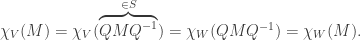
By character theory of compact groups, $V \cong W$ as K-reps. ♦

Now for the final piece of the puzzle.

Lemma 3. Let $f \in \mathbb{Z}[x_1, \ldots, x_n]$ be a symmetric polynomial. There are polynomial representations:

$\rho_1 : G\to GL(V_1),\quad \rho_2 : G\to GL(V_2),$

such that $\psi_{V_1} - \psi_{V_2} = f.$

Proof

Taking homogeneous parts, let us assume $f \in \Lambda_n^{(d)}$ for some degree $d\ge 0.$ Write f as a linear sum of elementary symmetric polynomials $\{h_\lambda\}_{\lambda\vdash d, \lambda_1 \le n}$ with integer coefficients; separating terms we have $f = g - h$ , where g, h are both linear combinations of $\{h_\lambda\}$ with non-negative integer coefficients. Hence, it suffices to show that $h_\lambda = \psi_V$ for some polynomial representation $G\to GL(V).$

Since $h_\lambda = h_{\lambda_1} \ldots h_{\lambda_l}$ , we can just pick:

$V = \left(\text{Sym}^{\lambda_1} \mathbb{C}^n\right) \otimes \left(\text{Sym}^{\lambda_2} \mathbb{C}^n\right) \otimes \ldots \otimes \left(\text{Sym}^{\lambda_d} \mathbb{C}^n\right),$

from the above. ♦

blue-lin

Consequences

Immediately we have:

Corollary 1. For any symmetric Laurent polynomial $f\in \mathbb{Z}[x_1^{\pm 1}, \ldots, x_n^{\pm 1}]$ , there exist rational representations:

$\rho_1 : G\to GL(V_1), \quad \rho_2 : G\to GL(V_2)$

such that $f = \psi_{V_1} - \psi_{V_2}.$

Proof

Indeed, 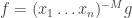$f = (x_1\ldots x_n)^{-M}g$ for some symmetric polynomial g in $x_1, \ldots x_n.$ Applying lemma 3, we can find $\rho_1, \rho_2$ such that $g = \psi_{V_1} - \psi_{V_2}$ ; now we take $\rho_1 \otimes \det^{-M}$ and $\rho_2\otimes \det^{-M}.$ ♦

Finally we have:

Corollary 2. Any irreducible K-module V can be lifted to a rational irreducible G-module.

Proof

By corollary 1, $\psi_V = \psi_{W} - \psi_{W'}$ where W, W’ are rational G-modules. Then $\psi_W = \psi_V + \psi_{W'} = \psi_{V\oplus W'}$ so $W\cong V\oplus W'$ as K-modules by lemma 2 above. By corollary 3 here, $V\subseteq W$ is a rational irreducible G-module. ♦

Summary of Results

Thus we obtain:

representations_correspondences_v2

Note the following.

When we consider virtual representations (recall that these are formal differences of two representations), this corresponds to all symmetric Laurent polynomials with integer coefficients.
Any rational G-representation is of the form $\rho \otimes \det^m$ where $\rho$ is a polynomial G-representation.

Moving Ahead

Our next task is to identify the irreducible rational G-modules V. Tensoring by some power of det, we may assume V is polynomial, so $\psi_V(x_1, \ldots, x_n)$ is a symmetric polynomial in $x_1, \ldots, x_n.$ Studying these will lead us back to Schur polynomials.

blue-lin

This entry was posted in Uncategorized and tagged character theory, general linear group, irreducible representations, matrix groups, representation theory, symmetric polynomials. Bookmark the permalink.

Leave a Reply Cancel reply

Enter your comment here...

Fill in your details below or click an icon to log in:

Email (required) (Address never made public)

Name (required)

Website

You are commenting using your WordPress.com account. ( Log Out / Change )

You are commenting using your Facebook account. ( Log Out / Change )

Connecting to %s

%d bloggers like this: