Introduction

Last year, I created a blog which was supposed to introduce concepts to abstract algebra in a systematic manner. Though I was reasonably happy with the end result, I got the sneaky feeling upon completion that the end product wasn’t any different from a typical textbook. The usual problems that plague students still remained. A friend of mine asked the critical question: “to whom are you targeting the notes at?” which set off an alarm. Indeed, the brevity of the notes indeed suggests that the reader is assumed to be relatively proficient, which would be a case of preaching to the choir.

This time, we’ll start by answering the above question.

The target audience is: students who’re interested in learning group theory, but who have little to no experience in concepts of abstract algebra.

What follows now is not a set of stand-alone notes, but a road map of topics to expect when studying group theory. We’ll try to motivate the definitions, theorems and examples as best as we can. We’ll be heavy on intuition and heuristics but low on rigour. Sometimes, instead of the most general statement possible, we’ll be content with a more concrete and down-to-earth version first.

The list of topics will be more or less the same as the above-mentioned blog. Repetitions will undoubtedly occur, since the important concepts are worth revising. Sometimes, we’ll also include comments that hint at stuffs deeper than those that are currently covered, hoping to entice our reader to learn more. So even if you feel reasonably competent in the topic, it may be worth a read.

In short, please don’t be scared off by any mention of unfamiliar/deep concepts.

Motivation (Permutations)

For this first chapter, we’ll be talking only about permutations. Readers who’re anxious to get to the meat of group theory should skip this article.

First, the primary concept which motivates study of groups is that of “symmetry” and “operations”. To fix concepts, we define the following.

Definition. A permutation of degree n to be a bijective map f : {1, 2, …, n} → {1, 2, …, n}.

We can compose two such maps as well as take the inverse of any such map to obtain another permutation. Let’s look at some common examples of permutations.

• The (perfect) riffle shuffle of a deck of cards is a fixed permutation of degree 52. [ Note: there are two ways to riffle-shuffle a deck, depending on whether the top card remains at the top or becomes the second card. ]
• A symmetry of a square ABCD is a permutation of degree 4 since it’s uniquely determined by where it takes the vertices. Let’s count the number of such symmetries, including reflections. Now, A can be mapped to any other vertex f(A). If we fix f(A), then the edge f(AB) has two possibilities since f(A) has two edges and both give valid symmetries. Thus there are 4 × 2 = 8 symmetries. For a greater challenge, try counting the number of symmetries of a regular icosahedron, making certain assumptions about the nature of the solid.
• Sam Loyd’s 15-puzzle corresponds to a permutation of degree 16 (since it permutes the 16 unit squares around, including the blank square). [ Note: purists would say that it forms a groupoid rather than a group, but let’s not worry about that now. ]
• The Topspin puzzle corresponds to permutations, typically of degree 20.
• A transformation of the Rubik’s cube is permutation of degree 9 × 6 = 54, by looking at how the unit squares move. [ Note: it’s actually possible to compute the exact number of transformations, via a powerful method called the Schreier-Sims algorithm. But that’d take us too far astray. ]

In order to provide a more economical notation for a permutation, we write it in a 2-row matrix form, e.g.:

can be expressed as

.

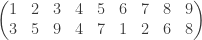
Or one can also express the same permutation in the form of cycles:

We usually write this as (1, 3, 9, 8, 6)(2, 5, 7), ignoring the fixed point 4.

The order of a permutation f is defined to be the smallest positive m for which is the identity map. Writing as disjoint cycles, it’s very clear that the order is merely the lcm of the length of the cycles. E.g. in the above permutation, the order is lcm(5, 3) = 15. We’ll like to cover two more concepts regarding permutations before moving on to abstract groups.

Exercise: what is the order of the riffle shuffle? [ Consider both variants. ]

Non-commutativity

Two permutations f and g are said to commute if fg = gf. It’s easy to find permutations which don’t commute, e.g. f(1) = 1, f(2) = 3, f(3) = 2 and g(1) = 2, g(2) = 1, g(3) = 3; the result is fg(1) = f(2) = 3 but gf(1) = g(1) = 2. Here, function composition always goes from right to left since fg(i) = f(g(i)).

Conjugate Permutations

This is based on the idea that relabeling the indices (1, 2, 3, 4) by, say, (a, b, x, y) does not substantially alter the nature of the permutations. So instead of the permutation f(1) = 1, f(2) = 3, f(3) = 4, f(4) = 2, we can write f(a) = a, f(b) = x, f(x) = y, f(y) = b, where the letters are dummy symbols here and not variables.

In particular, we can relabel (1, 2, 3, 4) by the same numbers, albeit permuted, say (3, 1, 4, 2). So the above permutation gets the relabeling:

Let’s do this carefully now. Suppose f : {1, 2, …, n} → {1, 2, …, n} is our original permutation. And g : {1, 2, …, n} → {1, 2, …, n} is the relabelling permutation. Now we list the entries of f as a graph or a lookup table, namely as a sequence of pairs:

Relabelling simply means that every single entry i in this list is replaced by g(i). So the new lookup table is:

From this, a moment of thought tells us that the new permutation is given by .

[ Note: I personally find the above picture of a lookup table conceptually helpful, especially when dealing with group actions on function spaces at higher levels. ]

Thus we define two permutations and to be conjugate if there is a permutation g such that . From the above explanation, it’s clear that two permutations are conjugate if and only if they have the same cycle structure, up to rearragement.

Example

Consider the two permutations of degree 9: 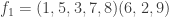and . Since both have two cycles, of lengths 3 and 5 respectively, the two permutations are conjugate. Now try to find a g such that . Question: how many such g are there?

Parity of a Permutation

We’ve already seen that every permutation is a product of disjoint cycles. So if we’re only equipped with cycles, we can obtain all permutations by successive compositions. [ Note: you’ll learn later that the technical term is: the set of cycles generates the group of permutations. ]

In fact, every cycle is a product of transpositions, where a transposition is a cycle of length 2, i.e. a swap (a, b) between two indices. E.g.:

.

Clearly, there’s more than one possible way to write a permutation as a product of transpositions. E.g. (1, 3) = (2, 3)(1, 2)(2, 3), so in fact, even the number of transpositions can vary. It’s thus a minor surprise that the parity of the number of transpositions is fixed.

Definition: a permutation is odd (resp. even) if it can be written as a product of an odd (resp. even) number of transpositions.

Hence, a permutation is either odd or even but not both. The proof is not hard: we count the number of cross-overs, i.e. the number of pairs (a, b) such that a < b but f(a) > f(b). It turns out each additional transposition will alter the number of cross-overs by an odd amount. Here it is if you’re interested.

Now, we can use this to solve Loyd’s 15-puzzle.

Loyd asked if it’s possible to swap the “14” and “15” tiles by a series of slides. The answer is no: the above permutation, of degree 16, is a transposition (14, 15) so it is an odd permutation. On the other hand, since the empty square is back to its original position, there must have been an even number of moves, and each move is a transposition (of the empty square “16” and some other piece), so the resulting permutation ought to be even. This creates a contradiction. ♦

There’s actually far more to be said about permutations, but we won’t dwell on them any further. Onward to group theory…